Upstream Notes 3: Multiplexed Single-Cell Sequencing? Meet cellranger multi

As discussed in the previous note, processing 10x Genomics data from multi-sample or multi-modal experiments (e.g., TCR/BCR + Gene Expression) typically involves cellranger multi for data processing and expression matrix generation. The "multi" here refers to either multiplex or multimodal — both widely used terms in modern biological research. Since multiplexing has broader applications, this article focuses primarily on that.
Introduction to Multiplexing
In the context of sequencing, multiplexing refers to the process of sequencing multiple samples simultaneously in a single sequencing run. It is an extremely common technique. When sample numbers are large, throughput requirements are high, or batch effects need to be minimized, multiplexing can substantially reduce sequencing costs and improve efficiency.
For example, without multiplexing, sequencing 10 samples might require 10 separate sequencing runs. With multiplexing, all 10 samples can be processed in a single run — saving significant time and money.
Specifically, multiplexing involves three main steps: labeling samples, pooling, and sequencing. The most critical step is the labeling, which makes it possible to later separate each sample's data. This separation process is called demultiplexing.
Working backwards from multiplexing, demultiplexing requires:
- Identifying the tag sequences in the raw sequencing data (also known as CMOs, cell multiplexing oligos, or HTOs, hashtag oligos).
- Assigning sequencing reads back to their original samples based on CMO identity.
- Performing further processing (alignment, quantification, etc.) on the assigned reads.
cellranger multi is the pipeline designed to carry out all of these steps.
CMO vs. Cell Barcode vs. UMI
After reading the above, you might be wondering: we already have cell barcodes and UMIs — why do we need CMOs? What exactly is the difference between CMOs, cell barcodes, and UMIs?
Let's start with a side-by-side comparison of their key characteristics:
| Feature | CMO | Cell Barcode | UMI |
|---|---|---|---|
| Purpose | Distinguish samples | Distinguish cells | Distinguish mRNA molecules |
| When added | Sample preparation | Single-cell isolation | Reverse transcription |
| Length | Short | Medium | Short |
| Location | Cell surface | 5′ end of cDNA | 5′ end of cDNA, after the cell barcode |
CMOs are oligonucleotides conjugated to antibodies or beads (or free-floating, without bead/antibody attachment). They carry specific sequence tags used to label distinct samples or cell populations. After mixing with the cell suspension, they bind to cells via magnetic or immunological interactions — BioLegend's TotalSeq series is a classic example.
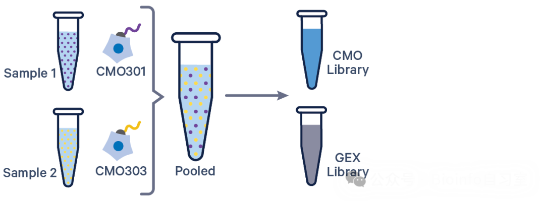
Example CMO configuration. Source: 10x Genomics
The Multiplexing Experimental Workflow
Let's walk through exactly how CMOs are used and how sequences are traced back to their original samples:
Sample labeling: At the start of the experiment, each sample is tagged with a unique CMO. These CMOs bind to proteins on the cell surface.
Single-cell isolation: When microfluidics is used to encapsulate individual cells into droplets (GEMs), the CMOs travel with the cells into the same droplet. Ideally, each droplet contains one cell (with its CMO), one gel bead (carrying cell barcodes and UMIs), and the reagents needed for reverse transcription.
Reverse transcription and PCR: Two reactions occur simultaneously within each droplet:
- a) CMOs are amplified and ligated to specific adapter sequences.
- b) Cellular mRNA is reverse-transcribed into cDNA and tagged with cell barcodes, UMIs, and adapter sequences.
Critically, both products (CMO-derived and cDNA-derived) share the same cell barcode.
Library preparation: After the reaction, droplets are broken and all products are pooled. At this stage, CMO and cDNA products are mixed together but can be distinguished by their characteristics: cDNA products are typically longer and contain gene-specific sequences, UMIs, and cell barcodes; CMO products are shorter and contain only the CMO-specific sequence and cell barcode.
Library separation: The size difference between CMO and cDNA products allows them to be physically separated by gel electrophoresis or magnetic bead purification. This step is essential — it enables the CMO and cDNA libraries to be processed independently.
Separate sequencing: The separated CMO and cDNA libraries are then sequenced individually.
Data analysis: During analysis, CMO sequencing data is processed first to establish a mapping between cell barcodes and sample origins. The cDNA sequencing data is then analyzed to obtain gene expression profiles for each barcode. Finally, the two pieces of information are integrated to reconstruct the gene expression landscape of individual cells from each sample.
This approach not only accurately separates cell data from different samples, but also allows the origin of every cell to be traced retrospectively during analysis — even though samples were pooled together at an early experimental stage. For example, if a given barcode corresponds to Sample A's CMO in the CMO data and to a particular gene expression profile in the cDNA data, we know that this expression profile comes from a cell in Sample A.
Hands-On with cellranger multi
Now that we understand the underlying principles of multiplexing, let's walk through how to actually run cellranger multi.
Preparing the Data
In addition to the Cell Ranger binary itself and a pre-downloaded reference genome, you'll need:
- Sequencing data: FASTQ files
- CMO sequences:
feature_reference.csv- Configuration file:
multi_config.csv
Sequencing Data
As mentioned above, the CMO and cDNA libraries in a multiplexing experiment are sequenced separately, so you'll receive two sets of FASTQ files:
fastq/
├── CMO/
│   ├── run1_CMO_L001_I1_001.fastq.gz
│   ├── run1_CMO_L001_I2_001.fastq.gz
│   ├── run1_CMO_L001_R1_001.fastq.gz
│   ├── run1_CMO_L001_R2_001.fastq.gz
│   └── ...
└── cDNA/
    ├── run1_cDNA_L001_I1_001.fastq.gz
    ├── run1_cDNA_L001_I2_001.fastq.gz
    ├── run1_cDNA_L001_R1_001.fastq.gz
    ├── run1_cDNA_L001_R2_001.fastq.gz
    └── ...
A quick refresher on FASTQ naming conventions:
SampleName_Lane (L001/L002/etc.)_Read (I1/I2/R1/R2)_Group (001).fastq.gz
I've deliberately renamed the FASTQ prefix to run1 to avoid confusion. In multiplexing experiments, the "sample" portion of the filename actually refers to a single sequencing run — it does not necessarily correspond one-to-one with biological samples. For instance, you might pool 6 samples and sequence them across two lanes of a single run. This would produce 8 CMO FASTQs (4 per lane: R1, R2, I1, I2) and 8 cDNA FASTQs — 16 files in total — even though the file names might all show the same "sample" prefix (e.g., run1). For comparison, if you sequenced those same 6 samples without multiplexing, you'd expect 6 × 4 = 24 FASTQ files — 8 more than the multiplexed approach.
CMO Reference File
In addition to the FASTQs, you need a CSV file listing each CMO's ID, the corresponding sample, the read in which it appears, the sequence pattern, the actual sequence, and the feature type.
As an example, suppose we use BioLegend's TotalSeq-A anti-mouse Hashtag series. These CMOs target the pan-cell-surface antigens MHC-I and MHC-II in mice to achieve broad coverage of both immune and non-immune cell types. After looking up the sequences from the product page, the feature_reference.csv looks like this:
id,name,read,pattern,sequence,feature_type
A0307,CMO1,R2,^(BC),GAGTCTGCCAGTATC,Multiplexing Capture
A0308,CMO2,R2,^(BC),TATAGAACGCCAGGC,Multiplexing Capture
A0303,PS1,R2,^(BC),CTTGCCGCATGTCAT,Multiplexing Capture
A0304,PS2,R2,^(BC),AAAGCATTCTTCACG,Multiplexing Capture
A0305,PSP1,R2,^(BC),CTTTGTCTTTGTGAG,Multiplexing Capture
A0306,PSP2,R2,^(BC),TATGCTGCCACGGTA,Multiplexing Capture
The id field here contains the product catalog number — it can technically be anything, as long as the sequence is correct. Similarly, the name field is freely customizable.
The read and pattern fields follow a specific format. For example, R2,^(BC) means the CMO sequence (barcode) is located at the beginning of Read 2 (^ is the regex anchor for the start of a string). This is the most common configuration, used by both 10x Genomics and BioLegend CMOs.
Of course, third-party CMOs may use different configurations. A few examples:
R1,(CB+BC): CMO follows the cell barcode, located in R1R1,(16C+8B): R1 contains a 16 bp cell barcode followed by an 8 bp CMOI2,^(BC): CMO is located at the start of the I2 read
And so on. The key elements to specify are: the read (R1/R2/I1/I2), the position (start ^, end $, or unspecified), the optional length, and the relative order of the cell sequence (C/CB) and CMO sequence (B/BC) (e.g., BC, CB+BC).
The sequence field is self-explanatory — just paste in the actual oligo sequence. For the feature_type field, use Multiplexing Capture for multiplexing experiments. For protein abundance measurements, use Antibody Capture instead. In that context, the oligo is no longer called a CMO but a feature barcode — CMOs are simply a specific type of feature barcode.
Configuration File
One key difference between cellranger multi and cellranger count is that all options and parameters must be specified in a separate CSV file rather than on the command line.
Here's an example multi_config.csv:
[gene-expression]
reference,refdata-gex-GRCm39-2024-A/
create-bam,true

[feature]
reference,feature_ref.csv

[libraries]
fastq_id,fastqs,feature_types
run1_cDNA,fastq/cDNA,Gene Expression
run1_CMO,fastq/CMO,Multiplexing Capture

[samples]
sample_id,cmo_ids
Sample1,A0307
Sample2,A0308
Sample3,A0303
Sample4,A0304
Sample5,A0305
Sample6,A0306
File Structure
The file is organized into sections, each beginning with a bracketed header: [gene-expression], [feature], [libraries], and [samples]. Each section contains key-value pairs specific to that section.
1. [gene-expression]
Configures parameters related to gene expression analysis.
Format:
- One parameter per line
- Format:
parameter_name,parameter_value
Available parameters:
reference,<path-to-reference>
chemistry,<chemistry-name>
expect-cells,<number>
force-cells,<number>
no-secondary,<true/false>
create-bam,<true/false>
...
Example:
[gene-expression]
reference,refdata-gex-GRCm39-2024-A/
create-bam,true
2. [feature]
Configures additional feature references, such as antibody/CMO sequences or CRISPR guide RNA sequences.
Format:
- Typically a single line pointing to the feature reference file
Example:
[feature]
reference,feature_ref.csv
3. [libraries]
Defines all sequencing libraries used in the experiment.
Format:
- First line is a header row defining column names
- Each subsequent line represents one library
- Columns are comma-separated
Required columns:
fastq_id: Unique identifier for the libraryfastqs: Path to the directory containing FASTQ filesfeature_types: Library type (e.g.,Gene Expression,Multiplexing Capture,Antibody Capture)
Example:
[libraries]
fastq_id,fastqs,feature_types
run1_cDNA,fastq/cDNA,Gene Expression
run1_CMO,fastq/CMO,Multiplexing Capture
4. [samples]
Defines the sample information. Note that the cmo_ids values must match the id column in your feature_reference.csv.
Format:
- First line is a header row
- Each subsequent line represents one sample
- Columns are comma-separated
Required columns:
sample_id: Sample identifiercmo_ids: The CMO ID(s) assigned to this sample
Example:
[samples]
sample_id,cmo_ids
Sample1,A0307
Sample2,A0308
Sample3,A0303
Things to Watch Out For
- The file must be in plain-text CSV format.
- Ensure all paths are correct — either relative or absolute paths will work.
- In the
[libraries]section, every library must have a uniquefastq_id. The CMO and cDNA libraries must be listed as separate entries. - The
cmo_idsvalues in[samples]must exactly match theidcolumn in yourfeature_reference.csv.
Running the Command
cellranger multi --id=cellranger_outs --csv=multi_config.csv --localcores=48 --localmem=128
With everything in place, the last step is simply to run cellranger multi! The key command-line options are:
--id: Experiment ID, which becomes the name of the output directory--csv: Path to the configuration CSV file (double-check the path!)--localcores: Number of CPU cores to use (48 in this example)--localmem: Memory limit in GB (128 GB in this example)
Understanding the cellranger multi Output
Once the run completes, cellranger multi generates multiple files and subdirectories in the specified output directory (cellranger_outs in this example). Here are the key outputs and what they contain:
outs/per_sample_outs/: Contains per-sample analysis results. For each sample, you'll find:filtered_feature_bc_matrix/: Filtered gene expression matrixraw_feature_bc_matrix/: Unfiltered (raw) gene expression matrixcloupe.cloupe: Loupe Browser visualization filemetrics_summary.csv: Summary of key QC metrics
outs/count/: Contains the combined count matrix and associated files across all samples.outs/multiplexing_analysis/: Contains the demultiplexing analysis results. The most important files are:assignment_confidence_table.csv: Per-cell confidence scores for sample assignmenttag_calls_summary.csv: Summary of cell counts and tag call statistics per sample
outs/multi/multiplexing_analysis.html: An interactive HTML report summarizing the multiplexing analysis, including sample assignment rates and labeling efficiency.outs/multi/gemgroup_*.html: Detailed HTML reports for each GEM group, including QC metrics and cell counts.outs/multi/config.csv: A copy of the configuration file used for this run.
For downstream analysis, the most commonly used outputs are:
- The filtered feature-barcode matrix (
filtered_feature_bc_matrix/): the primary input for clustering, differential expression, and other downstream analyses. - The sample assignment table (
assignment_confidence_table.csv): for determining which sample each cell belongs to. - The QC metrics summary (
metrics_summary.csv): for evaluating sequencing quality and overall experiment success. - The Loupe file (
cloupe.cloupe): for quick interactive visualization.
One more useful note: if you configured BAM file generation, you can use bamtofastq to reverse-generate per-sample FASTQ files from the BAM output. In other words, cellranger multi can also serve as a tool for demultiplexing and splitting individual sample FASTQs from a pooled run.
That's all for this installment — thanks for reading!
Originally posted on WeChat Official Account: bioinfo_studyroom