The New Azimuth Might Just Be the Best Cell Annotation Tool Out There

At Single Cell Genomics Day a few months ago (see the replay: Rahul Satija Summarizes 8 Key Developments in Single-Cell for 2025), the Satija Lab released their latest single-cell annotation package: Pan-Human Azimuth. In this post, we'll take a deep dive into this new tool with a hands-on walkthrough!
01
R Version: Installation & Usage
⚠️ Apple computers with M-series chips will throw errors when using the R package version. There is currently no workaround — consider using the Python version instead.
# Install from GitHub
devtools::install_github("satijalab/AzimuthAPI")
library(AzimuthAPI)
# Assuming your Seurat object is called obj
obj <- CloudAzimuth(obj)

# Annotation runs in the cloud, so local memory usage is minimal
# Once complete, the annotated obj is returned with results stored in meta.data
colnames([email protected])

...
[11] "full_hierarchical_labels"
[14] "final_level_labels"        "final_level_softmax_prob"  "full_consistent_hierarchy"
[17] "azimuth_broad"             "azimuth_medium"            "azimuth_fine"
[20] "azimuth_label"
Let's benchmark it (dataset: 16,222 cells × 20,262 genes; test platform: Ubuntu 24.04 LTS, 2× Intel Xeon E5-2690 v4 + entry-level Quadro K2200):
timing_result <- system.time({
    obj  <- CloudAzimuth(obj)
})

cat("User CPU time:", timing_result["user.self"], "seconds\n")
cat("System CPU time:", timing_result["sys.self"], "seconds\n")
cat("Total elapsed time:", timing_result["elapsed"], "seconds\n")

Running Pan-Human Azimuth on the cloud!
Uploading dataset
Uploading file and listening for updates...
File successfully uploaded
Running Pan-Human Azimuth:

Reference model and parameters:
Model name: M0.2
Evaluation batch size: 40960
Extract embeddings: True
Run umap: False
Refine labels in postprocessing: True
Integer counts detected by panhumanpy.ANNotate : False
Log-normalization performed by panhumanpy.ANNotate: False
Query object:
Total number of cells: 16222
Total number of features: 4528
Overlap w. feature reference: 4528 (~89%)

Splitting query data into 1 evaluation batches.

Running model:

  1/507 ━━━━━━━━━━━━━━━━━━━━ 5:09 611ms/step
...
507/507 ━━━━━━━━━━━━━━━━━━━━ 4s 6ms/step
Interpreting label predictions for consistent granularity at broad level.

Interpreting label predictions for consistent granularity at medium level.

Interpreting label predictions for consistent granularity at fine level.

Extracting azimuth embeddings:

  1/507 ━━━━━━━━━━━━━━━━━━━━ 22s 45ms/step
...
507/507 ━━━━━━━━━━━━━━━━━━━━ 2s 3ms/step

An object of class Seurat
4528 features across 16222 samples within 1 assay
Active assay: RNA (4528 features, 0 variable features)
1 layer present: data
1 dimensional reduction calculated: azimuth_embed
R script finished successfully
Output file ready for download
Downloading the output file...

User CPU time: 5.724 seconds
System CPU time: 0.595 seconds
Total elapsed time: 100.491 seconds
Comparing the annotation results against manual annotations, they're quite accurate. (Here I'm only showing the azimuth_broad level as an example — in practice there are three granularity levels from coarse to fine that you can choose from as needed.)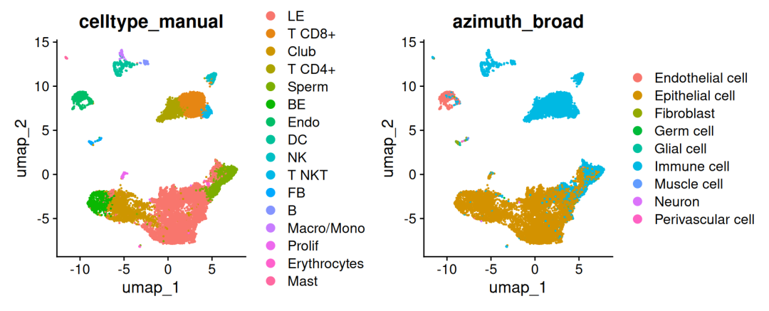 Result example
Here's a handy trick: since Azimuth annotates at the individual cell level, you can tally the cell types within each cluster and rank them by count to guide your final annotation decisions. This approach works with any cell-level annotation tool:
library(dplyr)
for(i in levels(obj$seurat_clusters)){
  print(paste("Cluster", i))
  [email protected] %>%
    filter(seurat_clusters == i)%>%
    # You can also use annotations at other granularity levels
    group_by(final_level_labels)%>%
    summarize(count = n())%>%
    arrange(desc(count))%>%
    head(n =5)%>%
    print()
}

[1] "Cluster 0"
# A tibble: 5 × 2
  final_level_labels                 count
  <chr>                              <int>
1 PIP mammary luminal cell            1035
2 Secretoglobin mammary luminal cell   317
3 Secretory cell                       219
4 CXCL2/3+ surface mucous cell         140
5 MMP7+ basal cell of bladder          137
[1] "Cluster 1"
# A tibble: 5 × 2
  final_level_labels    count
  <chr>                 <int>
1 GZMB CD8 T cell         531
2 Memory CD4 T cell       383
3 KLRB1 CD8 T cell        334
4 Memory CD8 T cell       294
5 GZMK+IL7R+ CD8 T cell   129
[1] "Cluster 2"
# A tibble: 5 × 2
  final_level_labels                 count
  <chr>                              <int>
1 Secretoglobin mammary luminal cell   454
2 PIP mammary luminal cell             314
3 Goblet cell                          176
4 Secretory cell                       129
5 CXCL2/3+ surface mucous cell          94
[1] "Cluster 3"
# A tibble: 5 × 2
  final_level_labels count
  <chr>              <int>
1 Cycling proB cell    140
2 Cycling preB cell    133
3 Secretory cell       127
4 Club cell             99
5 Memory CD8 T cell     99
[1] "Cluster 4"
# A tibble: 5 × 2
  final_level_labels                 count
  <chr>                              <int>
1 PIP mammary luminal cell             481
2 Secretory cell                       133
3 Tuft cell                            108
4 Secretoglobin mammary luminal cell    99
5 Goblet cell                           97
[1] "Cluster 5"
# A tibble: 5 × 2
  final_level_labels count
  <chr>              <int>
1 Memory CD4 T cell    301
2 Treg cell            219
3 CD4 T cell           121
4 Naive CD4 T cell      85
5 Memory CD8 T cell     81
In my experience, the immune cell annotations are remarkably accurate and authoritative. One important caveat: the reference dataset was built from healthy donors, so if results don't match your expectations, consider whether disease-related changes might be the cause.
02Python (Command Line) Version: Installation & Usage
The R package only supports cloud-based annotation, which can occasionally be unstable or suffer from connectivity issues. The Python version can run locally — either from the command line or in a Jupyter notebook. Note that the GPU-accelerated version requires CUDA, which is currently not supported on Mac.
# (Optional) Recommended: install into a dedicated conda environment with Python 3.9+
# conda create -n azimuth python=3.12
# conda activate azimuth

# Basic installation (CPU only)
pip install git+https://github.com/satijalab/panhumanpy.git

# GPU support (requires CUDA; not available on M-series Macs)
pip install 'git+https://github.com/satijalab/panhumanpy.git#egg=panhumanpy[gpu]'
Command Line Usage
# View options and help
annotate --help

# Run annotation — note that a new AnnData file obj_ANN.h5ad will be generated
annotate obj.h5ad
Let's time it:
time annotate obj.h5ad
Here are the benchmark results using the same dataset (16,222 cells × 20,262 genes) on two platforms (CPU only). If you have GPU resources, give the accelerated version a try!
# Ubuntu 24.04 LTS, Intel Xeon E5-2690 v4
real    1m20.639s
user    2m57.626s
sys    0m17.212s

# macOS Sequoia 15.5, M4
32.59s user
7.87s system
139% cpu
29.049 total
The speed is quite impressive — 1 minute 20 seconds on an aging server, and under 30 seconds on a Mac. For moderately sized datasets like this, running locally is actually faster than using the cloud.
Running in Python
You can also run the annotation directly within a Python environment.
import panhumanpy as ph
import anndata as ad

# View documentation (advanced API)
help(ph.AzimuthNN)

# View documentation (basic API)
help(ph.AzimuthNN_base)

# Read the AnnData object (you can also pass a file path directly)
obj = ad.read_h5ad("obj.h5ad")
To time the run in a Jupyter notebook, use the %%time magic command on the first line (skip it if you don't need timing):
%%time
# Build the AzimuthNN object
azimuth = ph.AzimuthNN(obj)
# Run annotation
azimuth.azimuth_refine()

# Extract annotation results
cell_metadata = azimuth.cells_meta
embeddings = azimuth.azimuth_embed()
umap = azimuth.azimuth_umap()

# Package the annotated AnnData and save
annotated_query = azimuth.pack_adata(save_path="obj_ANN.h5ad")
Timing results:
# Mac
CPU times: user 20.6 s, sys: 3.57 s, total: 24.2 s
Wall time: 16.1 s

# Server
CPU times: user 2min 9s, sys: 7.13 s, total: 2min 16s
Wall time: 54.4 s
Note that the AnnData structure after annotation differs from the original:
print("Data shape:", annotated_query.shape)
print("obsm keys:", list(annotated_query.obsm.keys()))
print("obs columns:", annotated_query.obs.columns.tolist()[:10])  # Show the first 10 column names

Data shape: (16222, 20262)
obsm keys: ['azimuth_embed', 'azimuth_umap']
obs columns: ['full_hierarchical_labels', 'level_zero_labels', 'final_level_labels', 'final_level_confidence', 'full_consistent_hierarchy', 'orig.ident', 'nCount_RNA', 'nFeature_RNA', 'scDblFinder.score', 'scDblFinder.weighted']
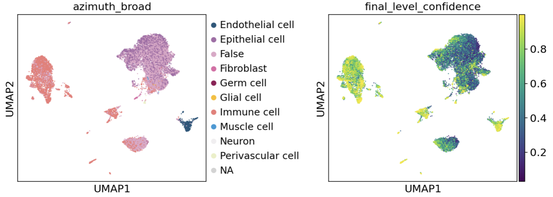
Let's visualize the results:
import scanpy as sc
annotated_query.obsm['X_umap'] = annotated_query.obsm['azimuth_umap']
sc.pl.umap(annotated_query, color=['azimuth_broad','final_level_confidence'],
           ncols=2, wspace=0.5)
03
Frequently Asked Questions
Here's a summary of the official FAQ:
What data types are supported?
Pan-Human Azimuth was trained on data from 23 human tissues: adipose tissue, adrenal gland, bladder, blood, bone marrow, brain, breast, eye, intestine, heart, kidney, liver, lung, lymph node, ovary, pancreas, placenta, skeletal muscle, skin, spleen, stomach, testis, and thymus.
- • The training dataset includes both single-cell RNA-seq (scRNA-seq) and single-nucleus RNA-seq (snRNA-seq) data, spanning multiple experimental platforms including droplet-based, plate-based, and combinatorial indexing technologies.
- • Cancer datasets were excluded during training.
- • In general, query datasets that fall within the scope of the above parameters should yield good annotation results with Pan-Human Azimuth.
What preprocessing steps are required?
- • The R interface requires a Seurat object as input; the Python interface requires an AnnData object.
- • Users should perform quality control before annotation (i.e., filter cells based on UMI counts and mitochondrial gene percentage thresholds).
- • R users need to perform standard log-normalization with
NormalizeDataprior to annotation — see the official tutorial for details. - • Python users can either normalize beforehand or provide raw integer counts (the package will handle normalization automatically).
- • Variable gene selection is not required — users should retain all quantified genes in the object before annotation.
What does the package output?
- • full_hierarchical_labels: Hierarchical cell type annotations with predictions at multiple levels of the cell type taxonomy. Example: Immune cell | Lymphocyte | T/NK cell | T cell | CD4 T cell | Naive CD4 T cell
- • final_level_softmax_prob: Prediction probabilities associated with the hierarchical labels.
- • azimuth_embed: 128-dimensional cell embeddings generated by the neural network encoder, which are decoded to produce annotation results.
- • For easier interpretation, labels are post-processed to be more concise and readable, with granularity levels standardized across cells. These include
final_level_labels,azimuth_fine,azimuth_medium, andazimuth_broad. See the official tutorial for details.
How should I QC the annotation results?
- •
final_level_softmax_probis a useful QC metric. We typically exclude cells with scores < 0.5. - • No QC metric is perfect, so we strongly recommend identifying and visualizing differentially expressed genes for each annotated cell population as a manual sanity check. To help with this, the R API package provides the
make_azimuth_QC_heatmapsfunction, demonstrated in the tutorial.
Can Pan-Human Azimuth annotate disease data?
Yes. We routinely use Pan-Human Azimuth to annotate disease data. In many — if not most — cases, malignant cells still retain partial molecular signatures of their normal counterparts. Reference mapping workflows, including Pan-Human Azimuth, are widely used to annotate both healthy and diseased cells to a common set of cell types, followed by within-cell-type differential expression analysis to identify malignant transformations.
However, the Pan-Human Azimuth reference does not include disease-specific cell types. Malignant cells will be mapped to the most similar normal cell type. The QC measures discussed above help ensure that these annotations remain useful for comparison with healthy samples and for identifying disease-specific signatures.
The Pan-Human Azimuth training dataset does not contain cancer samples. Tumor cells often undergo substantial molecular reprogramming that diverges significantly from normal cells, which may lead to poor mapping performance.
Is there a size limit for mappable datasets?
- • Both R and Python workflows are highly scalable. The R workflow runs in the cloud at approximately 50,000–100,000 cells/minute. The Python workflow achieves similar throughput on a standard laptop.
- • Pan-Human Azimuth annotates and embeds each cell independently, so large datasets can be chunked and mapped serially. Using this strategy, we mapped over 80 million cells from the scBaseCamp repository in less than a day.
Future Plans
Yes! We're excited about upcoming features, including:
- • Improved quality control: Enhanced QC metrics with better calibration than softmax probabilities, capturing uncertainty across multiple levels of the hierarchy.
- • Low-quality cell detection: In the current version, low-quality cells (e.g., those with UMI < 100) tend to map to cell types with inherently low RNA content, such as plasma cells and αβT (entry) cells. We are working to explicitly flag these as low quality in future releases.
- • Higher-resolution annotations: We are continuously updating the reference dataset to provide finer-grained annotations and incorporate more recently discovered cell types.
References
- 1. https://satijalab.org/pan_human_azimuth/
- 2. R tutorial: https://satijalab.org/panhuman_r_vignette
- 3. Python tutorial: https://github.com/satijalab/panhumanpy/blob/main/tutorial_panhumanpy.ipynb
04
Afterword
We previously published an article on using large language models to assist with single-cell annotation: The Future Is Here: The Era of LLM × Single-Cell Has Begun. What do you think is the future of single-cell annotation — reference-based approaches or large language models? What's the best annotation tool you've used? Let us know in the comments! To stay updated with our study notes, give us a ✨:
Past highlights ⬇️:
Publication-Quality RNA-seq Figures with tidyplots: A Practical Guide
Stop Using .rds for Single-Cell Data — Try qs Instead!
STAR Has a Bug?? A Full Post-Mortem
Originally posted on WeChat Official Account: bioinfo_studyroom