Statistics Self-Help Guide 3: The p-value and t-test You've Probably Never Fully Understood
As experimentalists, we constantly need to judge whether a result is "real." Statistical software hands us a mysterious p-value, but what does that number actually mean? Today, we'll use the most basic statistical test — the one-sample t-test — to thoroughly demystify the logic of hypothesis testing.
Is the Difference Real?
You're running a Western blot to measure the expression level of a particular protein. Based on prior experience and the literature, the normal expression level of this protein should be 10. But today you measured a value of 12.
The question is: is this difference real, or is it just experimental noise?
That is exactly what hypothesis testing is designed to answer.
Building an Imaginary World — the Null Hypothesis
To address this question, statisticians devised a clever strategy: proof by contradiction.
We start by assuming "nothing happened" — that the value of 12 you measured is simply the result of normal fluctuation around the true value of 10. This assumption is called the null hypothesis (H₀).
Think of it this way: if the protein's true expression level really is 10, what would you get if you repeated the measurement 1,000 times? Due to pipetting error, antibody lot-to-lot variability, exposure time fluctuations, and other sources of noise, you'd get a cloud of values scattered around 10 — perhaps 9.8, 10.2, 9.5, 10.7… The distribution formed by all these values is the null distribution.
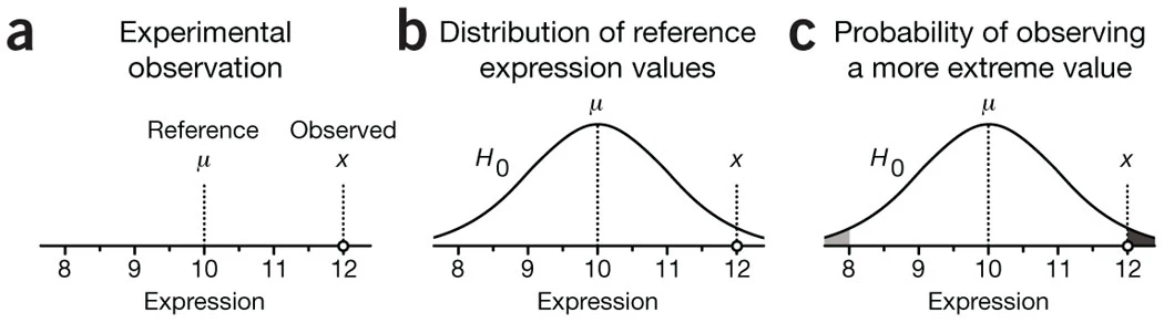
Figure 1 | The basic logic of hypothesis testing. (a) Our observed value is x = 12, and the known reference value is μ = 10. (b) We assume a null distribution representing all possible measurement outcomes when the protein's true expression is 10, centered at μ. (c) The p-value equals the total area under this null distribution in regions more extreme than our observed value.
The p-value: A Frequently Misunderstood Probability
Here is the key question: if the protein's true expression really is 10, how likely are we to measure a value as extreme as 12 (or more extreme)?
That probability is the p-value.
An analogy: suppose someone claims they can control coin tosses. They flip a coin 10 times and get 9 heads. If the coin is fair (null hypothesis), the probability of such an extreme result is very small (small p-value). So we're inclined to believe they might genuinely have some special trick (we reject the null hypothesis).
The Biggest Pitfalls Around p-values
Pitfall 1: Does p = 0.05 mean there's only a 5% chance the null hypothesis is true?
Absolutely not! The p-value is calculated assuming the null hypothesis is 100% correct. It tells you how surprising the data would be if there were no effect — it is not the probability that an effect exists.
Pitfall 2: The smaller the p-value, the larger the effect?
Not necessarily! With a large enough sample size, even a trivially small, biologically meaningless difference can yield an extremely small p-value. For example, two antihypertensive drugs whose effects differ by just 0.1 mmHg might produce p < 0.001 with 10,000 patients — yet that 0.1 mmHg difference is clinically irrelevant.
Pitfall 3: p > 0.05 proves there is no difference?
Wrong! "No evidence of a difference" ≠ "evidence of no difference." The non-significant result may simply reflect insufficient sample size or excessive experimental noise.
Pitfall 4: p = 0.05 is an inviolable threshold?
Too dogmatic! p = 0.049 and p = 0.051 represent essentially the same strength of evidence. Treating 0.05 as the dividing line between truth and falsehood is not scientifically justified.
Replicate Experiments: Making Conclusions More Reliable
A single measurement is prone to false alarms. So we repeat the experiment — say, five times — to obtain a set of data.
We then use:
- The sample mean (x̄ = 10.85) to estimate the true expression level
- The sample standard deviation (s
x= 0.96) to quantify the spread of the data - The standard error of the mean (s
x/√n) to assess how precisely the mean is estimated
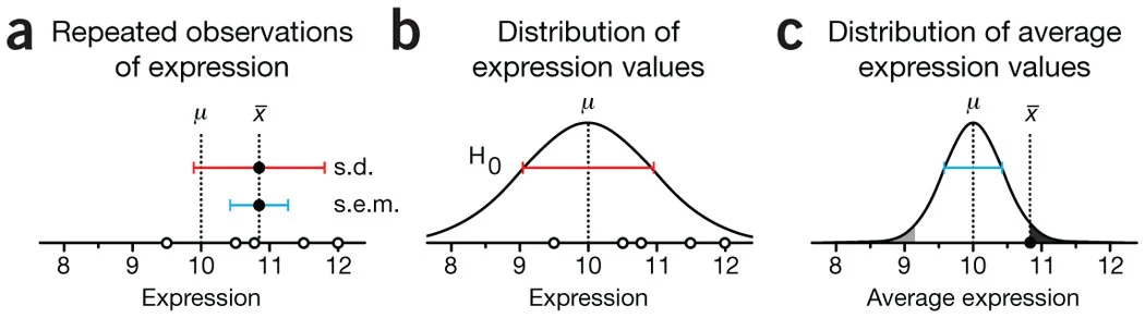
Figure 2 | Statistical testing using a sample. (a) n = 5 independent replicates, yielding the sample mean and standard deviation. (b) The null distribution is modeled as a normal distribution, its standard deviation estimated from the sample. (c) The p-value is the extreme-tail area of the sampling distribution of the mean, whose spread equals the s.e.m.
The t-statistic: A Standardized Measure of Difference
To make comparisons consistent across contexts, we compute a standardized measure called the t-statistic:
t = (sample mean − reference value) / standard error
  = (x̄ − μ) / (s_x / √n)
Plain-language interpretation: the t-statistic tells you how many standard errors the observed difference represents. t = 2 means the observed deviation is twice the size of the standard error.
Why the t-Distribution Instead of the Normal Distribution?
There is an interesting story here. In the early twentieth century, a chemist named William Gosset working at the Guinness brewery in Dublin noticed a problem: with small samples, using the normal distribution is "overly optimistic."
The reason is simple: the standard deviation of a small sample tends to underestimate the true variability of the population. It's like interviewing only five people to estimate the average height of an entire country — by chance, those five might all be similar in height, causing you to underestimate how variable people's heights actually are.
To compensate for this underestimation, Gosset (writing under the pen name "Student") proposed the t-distribution — it looks like a normal distribution, but with heavier tails.
What "Heavier Tails" Means
The t-distribution assigns higher probability to extreme values than the normal distribution does. This is a deliberately conservative approach — better to miss a few real effects than to report spurious ones.
A concrete example:
- Using the t-distribution: t = 1.98, p = 0.119 (not significant)
- Incorrectly using the normal distribution: t = 1.98, p = 0.048 (significant)
See the difference? Skipping the t-distribution can lead you to a false "significant" conclusion.
The Effect of Sample Size
The shape of the t-distribution is governed by its degrees of freedom (d.f. = n − 1):
- Small sample (e.g., n = 5) → t-distribution has very heavy tails → stronger evidence required to reach significance
- Large sample (e.g., n > 30) → t-distribution converges toward the normal distribution → because large-sample standard deviation estimates are more accurate
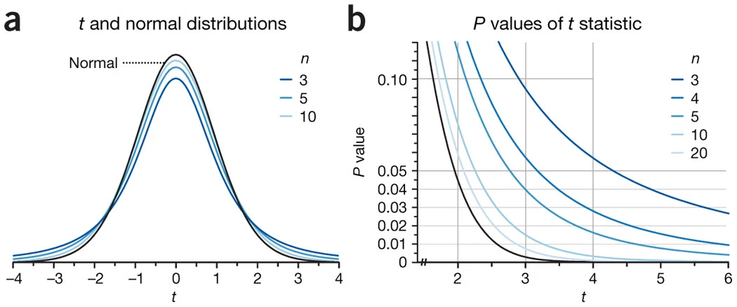
Figure 3 | The t-distribution vs. the normal distribution. (a) The t-distribution has heavier tails than the standard normal, assigning higher probability to extreme values. Its shape is determined by degrees of freedom (n − 1); as n grows, it approaches the normal. (b) For the same t-value, the p-value is larger (less significant) when n is small.
Confidence Intervals: A Different Perspective
Beyond the p-value, we can also ask: what range of reference values would be consistent with our data?
This is the 95% confidence interval. If it comes out to [9.66, 12.04], that means:
- If the true value lies anywhere between 9.66 and 12.04, our sample would not show a statistically significant difference.
- This interval conveys information about the plausible size of the effect — far more useful than a simple "significant / not significant" verdict.
Practical Tips
When to Use the One-Sample t-Test
- Comparing a sample mean against a known reference or standard value
- Testing whether a product meets a quality specification
- Validating the accuracy of an experimental method
- Assessing whether gene expression deviates from a normal baseline level
Assumptions
- Data should be approximately normally distributed (especially important with small samples)
- Observations must be independent (not repeated measurements of the same sample)
- A clearly defined reference value must exist (from the literature, a standard, or a control group)
How to Report Results Correctly
❌ Wrong: "P < 0.05, the result is significant, confirming our hypothesis."
✅ Correct: "Compared to the reference value (μ = 10), we observed a difference in expression level (mean = 10.85, SD = 0.96, n = 5, t = 1.98, P = 0.119) that did not reach statistical significance at α = 0.05."
Final Thoughts
The one-sample t-test is the entry point for statistical inference, but the ideas it embodies run through all of statistics:
- Think by contradiction (the null hypothesis)
- Quantify uncertainty (the p-value)
- Account for sample size (the t-distribution)
- Distinguish statistical significance from practical importance
Remember: p-values are a tool, not the goal. What truly matters is understanding the biological story your data is telling you.
Statistical significance ≠ biological importance
Large sample ≠ good study
P < 0.05 ≠ truth
Stay critical. Let statistics serve science — not the other way around.
Reference:
Krzywinski, M. & Altman, N. (2013). Points of significance: Significance, P values and t-tests. Nature Methods, 10(11), 1041–1042.
Originally posted on WeChat Official Account: bioinfo_studyroom