Statistics Self-Help Guide 1: Embracing Uncertainty
A while ago, when updating my qPCR tool (see qPCR Tool Update!), I discovered a mistake I had made — namely, running ANOVA on non-normally distributed fold-change values. While correcting the error, I began to take a fresh look at some of the statistical concepts that are commonly overlooked or confused in scientific research. That's how this Statistics Self-Help Guide series was born. For the first instalment, let's talk about uncertainty.
If you've ever done bench work, you've surely faced these existential questions:
- Why do I get slightly different Ct values every time I repeat the same qRT-PCR — even when I follow the protocol exactly three times?
- Why do my two biological replicates show such wildly different gene expression levels when the sequencing data comes back?
- When I claim a gene is "upregulated" based on sequencing results, how reliable is that conclusion, really?
Behind all of these lies a spectre — randomness. Statistics is the only tool we have to tame this spectre. It doesn't tell us "right" or "wrong"; instead, it tells us "how likely we are to be wrong".
This post is adapted from the classic explainer series Points of Significance in Nature Methods. The goal is to use the most accessible language possible to help you build the statistical thinking that is essential for bioinformatics analysis.
Can You Really Trust Your Research Intuition?
Before diving into statistics, let's play a game — and see just how fragile our brains are when it comes to probabilities.
The Monty Hall Problem
- There are three doors on stage. Behind one is a sports car; behind the other two are goats.
- You choose Door 1 (giving you a 1/3 chance of winning).
- The host, who knows where the car is, opens Door 3 to reveal a goat — thereby eliminating one wrong answer.
- Now the host gives you a choice: stick with Door 1, or switch to Door 2?
What's your gut reaction? Does it feel like there's an equal 50/50 chance either way?
The correct answer is: switch! By switching to Door 2, your probability of winning jumps from 1/3 to 2/3!
Feels counter-intuitive, right? When this answer was first published, it provoked fierce opposition from thousands of readers — including many PhDs. This simple example demonstrates a brutal truth: when facing uncertainty, intuition often deceives us. When handling complex biological data, we need the "power-up" of statistics to guide our decisions even more.
The Two Worlds of Statistics: Description and Inference
In simple terms, statistics can be divided into two domains:
Descriptive Statistics
- Purpose: To "summarise". It uses a few key metrics — such as the mean and standard deviation (SD) — to paint a picture of the data.
- Example: Calculating the average expression level and the range of variation for a particular gene across your 10 samples.
Inferential Statistics
- Purpose: To "generalise". Starting from limited data at hand (a sample), you draw conclusions about a much larger reality (the population).
- Example: Using sequencing data from 10 liver cancer patients to infer the expression pattern of a gene across all liver cancer patients. This is the core objective of scientific research.
The bridge connecting these two worlds is sampling.
From "Population" to "Sample": The Art of Seeing Through a Keyhole
To understand inference, you first need to grasp two core concepts: the population and the sample.
- Population: The complete set of all subjects of interest. For example, the liver cells of every healthy person on Earth, or every possible gene transcript from a given species. A population has its "true" parameters, which are usually impossible to measure directly, such as:
- Population mean μ: Describes the average level of the population.
- Population standard deviation σ: Describes the degree of variation among individuals in the population.
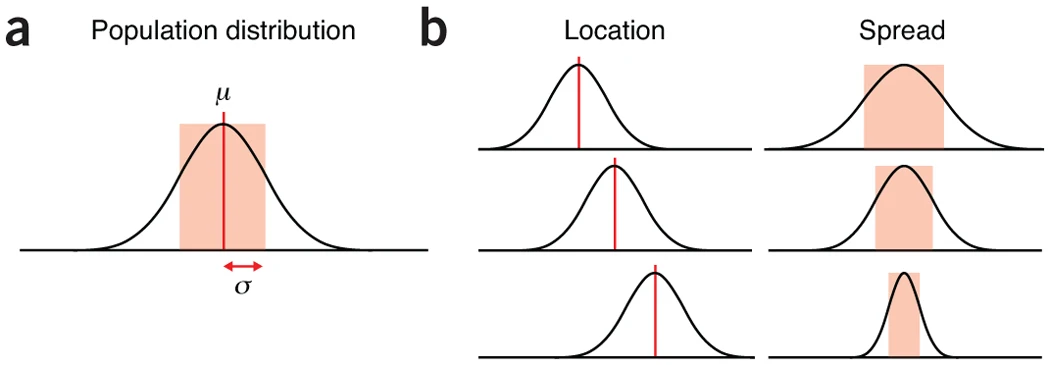 Figure 1
Figure 1 explained: (a) Suppose this is the expression-level distribution of a certain gene across all cells; the red line marks its true mean μ. (b) μ determines the "location" of the distribution, while σ determines how "wide" or "narrow" it is.
- Sample: A small subset of data we actually observe from the population. For example, your 3 sequencing replicates, or the 100 cells you examine under a microscope. Samples have corresponding statistics:
- Sample mean x̄ (read as "X-bar")
- Sample standard deviation s
The starting point of all our analyses is using the sample's x̄ and s to estimate the population's μ and σ.
❗️Key point: For this estimate to be reliable, your sample must be representative of the population. The most common approach is random sampling — ensuring every member of the population has an equal chance of being selected. A biased selection (e.g., only picking the healthy-looking cells) will cause all your conclusions to deviate from the truth.
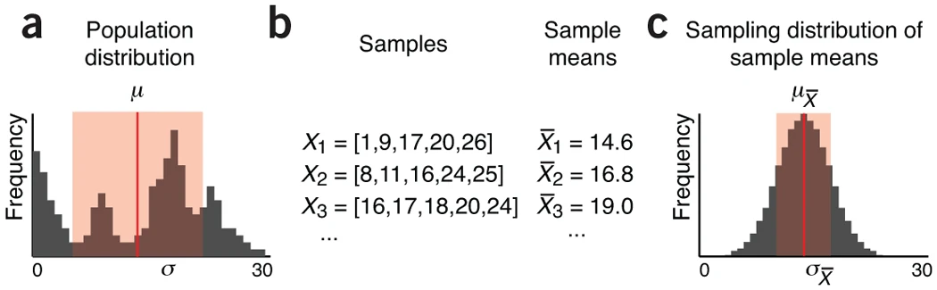 Figure 2
Figure 2 explained: (a) This is a population distribution we cannot fully observe. (b) We draw three different random samples from it; each sample yields its own sample mean. (c) If we could collect the sample means from every possible sample, their distribution would form the "sampling distribution of the sample mean".
The "Divine Theorem" of Statistics: The Central Limit Theorem
You might worry: my samples are all over the place — how can I possibly use them to infer anything about the population? Fear not — one of the most important and magical theorems in statistics, the Central Limit Theorem (CLT), has your back.
The core idea of the CLT:
No matter what your population distribution looks like — whether normal, uniform, or wildly irregular — as long as your sample size n is large enough, the distribution of the sample means will approximate a normal distribution (the classic bell-shaped curve).
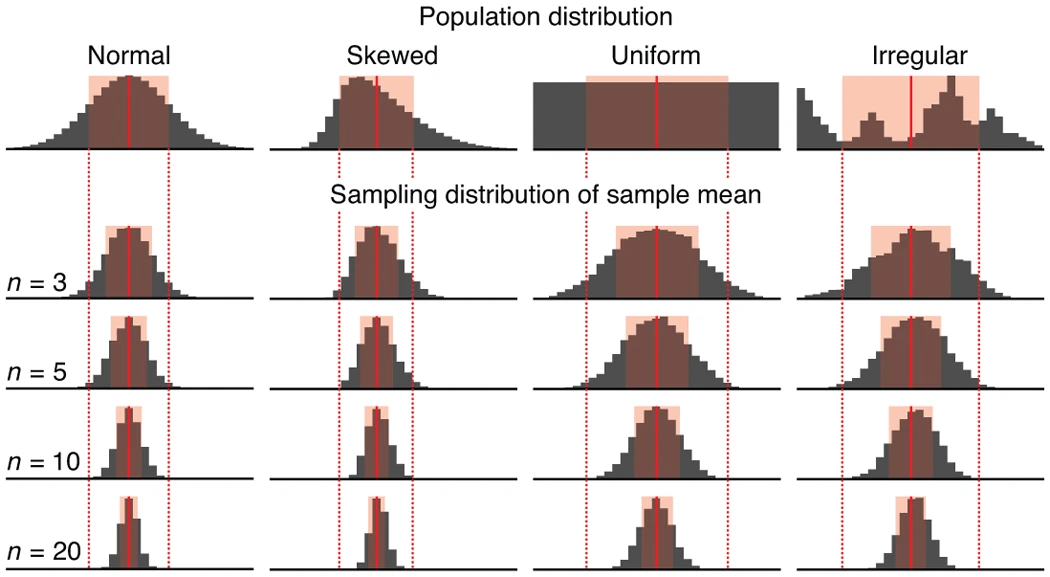 Figure 3
Figure 3 explained: Even if the original population distribution is skewed, uniform, or irregular, as the sample size n increases (from 3 to 20), the distribution of sample means (lower rows) increasingly resembles a standard normal distribution.
The CLT also tells us two key parameters of this "sampling distribution of the mean":
- Its mean equals the population mean μ.
- Its standard deviation equals σ/√n.
This σ/√n has a more well-known name: the Standard Error of the Mean (SEM).
Standard Deviation (SD) vs. Standard Error (SEM): Can You Really Tell Them Apart?
This is a notorious source of confusion for researchers — so let's set the record straight:
Standard Deviation (SD, symbol σ or s)
- Describes: The spread of your data itself.
- Answers the question: "How much do the values among my biological replicates vary?"
- Use case: Primarily for descriptive statistics — it tells you how wide or narrow the data distribution is.
Standard Error of the Mean (SEM, symbol σ/√n)
- Describes: How far your calculated sample mean might be from the true population mean. In other words, it measures the precision of your estimate.
- Answers the question: "How confident am I that the mean from this experiment is close to the real-world mean?"
- Use case: Primarily for inferential statistics — commonly used for error bars in figures to convey the confidence of the mean estimate.
In short: SD describes data variability; SEM describes the precision of the mean.
The Cost of Precision: Why "More Effort" Doesn't Always Equal "Better Results"
From the SEM formula σ/√n, we can uncover a harsh truth:
Increasing the sample size n improves precision only by its square root — in other words, there are diminishing marginal returns.
Example: Suppose you go to great effort to increase your biological replicates from 3 to 6, doubling the sample size. Your estimation precision (measured by SEM) only improves to 1/√2 ≈ 71% of the original.
To double your precision (halve the SEM), you need to quadruple the sample size! (For example, going from 3 replicates to 12!)
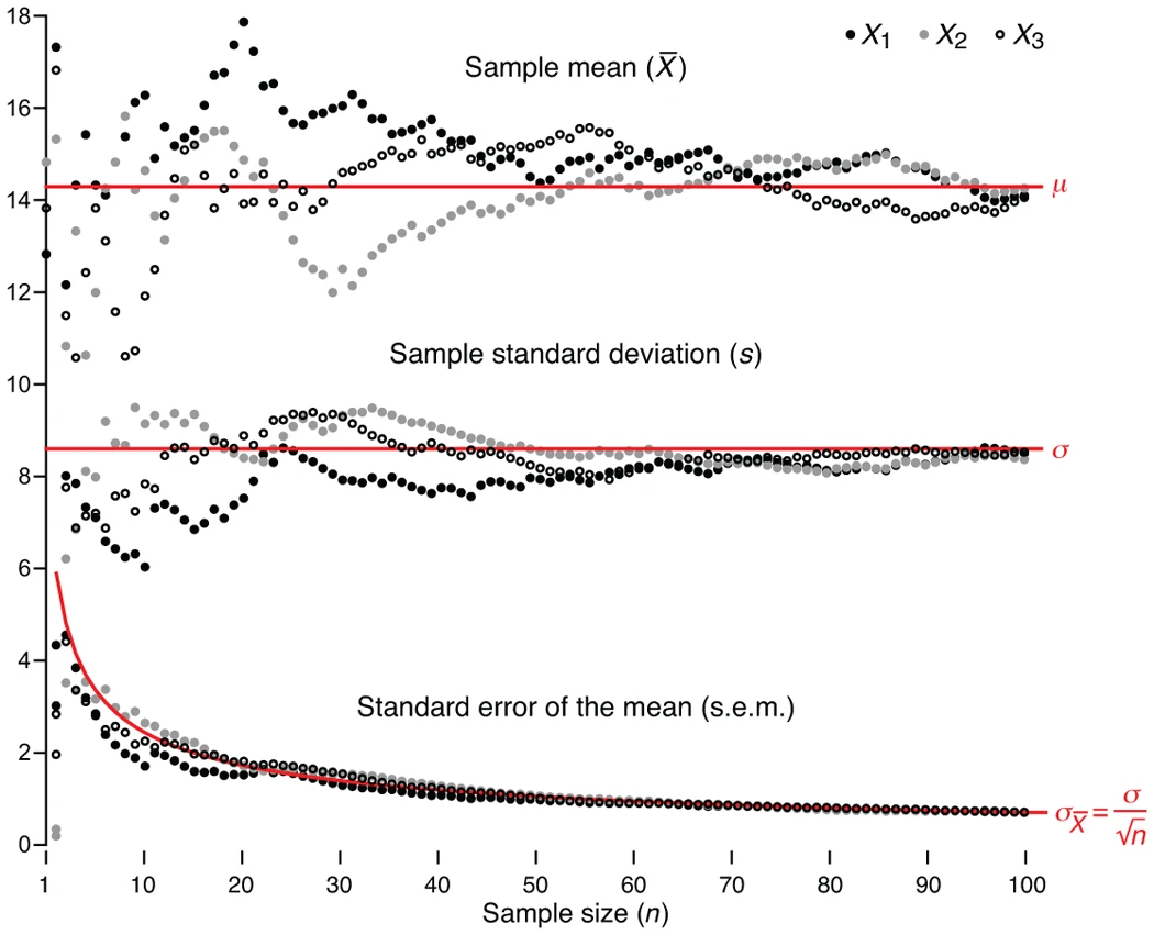 Figure 4
Figure 4 explained: As the sample size n increases, the sample mean (x̄, top curve) and sample standard deviation (s, middle curve) gradually converge and stabilise near the true population values (red lines). The standard error (SEM, bottom curve) decreases following the √n rule — steadily but ever more slowly.
This √n rule is the "cost-effectiveness principle" you must keep in mind when designing experiments and deciding how many samples to measure.
Key Takeaways
Statistics is not a pile of daunting formulas — it is a way of thinking. When working with high-throughput data, remember:
Embrace uncertainty: Never treat your measurements (e.g., a gene's TPM = 150) as absolute truth. They are only estimates. Acknowledging and quantifying uncertainty is the hallmark of the scientific spirit.
Beware of small samples: When biological replicates are scarce (e.g., n = 2 or 3), your sample mean may be far from reality. Always be cautious when interpreting results.
Understand the cost of precision: When pursuing greater statistical power, weigh the cost of adding more samples against the actual gain in precision. The √n rule means "brute force" won't always work miracles.
Distinguish SD from SEM: When reading papers or drawing figures, always be clear about whether the error bars represent SD or SEM. The former shows data variability; the latter shows mean precision — the two convey fundamentally different information.
Our goal is not to eliminate uncertainty, but to scientifically quantify and manage it. By understanding today's content, you've already taken the crucial first step from "data analyst" to "data scientist".
Coming up next: We'll go deeper and explore how to use confidence intervals to delineate uncertainty more intuitively, and how to correctly draw and interpret error bars. Stay tuned!
Reference: Krzywinski, M. & Altman, N. Importance of being uncertain. Nature Methods 10, 809-810 (2013).
Originally posted on WeChat Official Account: bioinfo_studyroom