Single-Cell Analysis with Theis Lab: How Many Cell Annotation Strategies Do You Know?

Single-Cell Best Practices

Cell Annotation

Chapter Overview — SECTION PREVIEW

1. Core concepts and biological significance of cell annotation
2. Manual annotation strategies using marker genes
3. Principles and applications of automated annotation tools
4. Advanced annotation via reference mapping
5. Hands-on practice: combining multiple strategies for cell annotation

This section corresponds to Chapter 11: Annotation in the original book.

In single-cell sequencing analysis, we work with gene expression data from tens of thousands of individual cells. But raw data alone is not enough — we need to know the identity of each cell, i.e., what cell type it belongs to. This process of assigning labels to cells is what we call cell annotation.

Biologists use the term "cell type" to describe populations of cells that share specific functions and express particular marker genes. For example, plasma B cells are antibody-secreting white blood cells that can be identified by a defined set of marker genes.

Like any classification system, however, cell type boundaries are sometimes fuzzy. On one hand, advances in technology have allowed researchers to resolve increasingly fine subtypes or states — T cells, for instance, can be further split into activated and resting populations. On the other hand, certain lineages form a continuum rather than discrete categories: during hematopoiesis, cells gradually differentiate from stem cells into diverse immune cell types, with no clear-cut boundaries.

Consequently, the distinctions between "cell type," "subtype," and "cell state" often carry a degree of subjectivity. In recent years, the broader term cell identity has gained traction as a way to sidestep rigid classifications.

Setup

First, let's set up the environment.

import warnings
warnings.filterwarnings("ignore", category=DeprecationWarning)

import scanpy as sc
import pandas as pd
import numpy as np
import os
from scipy.sparse import csr_matrix
import seaborn as sns
import matplotlib.pyplot as plt
import celltypist
from celltypist import models
import scarches as sca
import urllib.request

# Set figure parameters
sc.set_figure_params(figsize=(5, 5))

Next, load the bone marrow dataset used in the previous section:

adata = sc.read(
    filename="s4d8_clustered.h5ad",
    backup_url="https://figshare.com/ndownloader/files/41436666",
)

Strategy 1: Manual Annotation

In the early days of single-cell analysis, the most common annotation approach relied on marker genes.

Researchers compile a list of genes known to be associated with particular cell types, and then infer cell identity for each cluster based on the expression patterns of those genes.

Advantages of this approach:

• Simple and intuitive; particularly efficient for early FACS-based data (which typically profiled only a few dozen genes)
• Transparent and easy to interpret

Drawbacks:

• Many cell types lack truly unique marker genes
• The same marker may behave inconsistently across datasets
• Combining multiple genes or setting expression thresholds introduces subjectivity

For these reasons, the standard practice is to first cluster cells and then assign labels at the cluster level, rather than annotating cell by cell. This is not only more robust, but also helps mitigate the dropout problem inherent in single-cell transcriptomics.

In general, manual annotation follows two complementary approaches:

1. Marker-first (marker → cluster): Start with a curated list of markers for expected cell types, then examine their distribution across clusters in your data.
2. DEG-first (cluster → marker): First compute differentially expressed genes (DEGs) for each cluster, then look up which known cell types those genes correspond to.

Let's begin with the marker-first approach.

Defining Known Markers

Here we define a curated marker gene table for bone marrow cell types, compiled from the literature:

marker_genes = {
    "CD14+ Mono": ["FCN1", "CD14"],
    "CD16+ Mono": ["TCF7L2", "FCGR3A", "LYN"],
    "ID2-hi myeloid prog": ["CD14", "ID2", "VCAN", "S100A9", "CLEC12A", "KLF4", "PLAUR"],
    "cDC1": ["CLEC9A", "CADM1"],
    "cDC2": ["CST3", "COTL1", "LYZ", "DMXL2", "CLEC10A", "FCER1A"],  # DMXL2 is a negative marker
    "Normoblast": ["SLC4A1", "SLC25A37", "HBB", "HBA2", "HBA1", "TFRC"],
    "Erythroblast": ["MKI67", "HBA1", "HBB"],
    "Proerythroblast": ["CDK6", "SYNGR1", "HBM", "GYPA"],  # HBM, GYPA are negative markers
    "NK": ["GNLY", "NKG7", "CD247", "GRIK4", "FCER1G", "TYROBP", "KLRG1", "FCGR3A"],
    "ILC": ["ID2", "PLCG2", "GNLY", "SYNE1"],
    "Lymph prog": ["VPREB1", "MME", "EBF1", "SSBP2", "BACH2", "CD79B", "IGHM", "PAX5", "PRKCE", "DNTT", "IGLL1"],
    "Naive CD20+ B": ["MS4A1", "IL4R", "IGHD", "FCRL1", "IGHM"],
    "B1 B": ["MS4A1","SSPN","ITGB1","EPHA4","COL4A4","PRDM1","IRF4","CD38","XBP1","PAX5","BCL11A","BLK","IGHD","IGHM","ZNF215"],  # IGHD, IGHM are negative markers
    "Transitional B": ["MME", "CD38", "CD24", "ACSM3", "MSI2"],
    "Plasma cells": ["MZB1", "HSP90B1", "FNDC3B", "PRDM1", "IGKC", "JCHAIN"],
    "Plasmablast": ["XBP1", "RF4", "PRDM1", "PAX5"],  # PAX5 is a negative marker
    "CD4+ T activated": ["CD4", "IL7R", "TRBC2", "ITGB1"],
    "CD4+ T naive": ["CD4", "IL7R", "TRBC2", "CCR7"],
    "CD8+ T": ["CD8A", "CD8B", "GZMK", "GZMA", "CCL5", "GZMB", "GZMH", "GZMA"],
    "T activation": ["CD69", "CD38"],  # CD69 is more reliable
    "T naive": ["LEF1", "CCR7", "TCF7"],
    "pDC": ["GZMB", "IL3RA", "COBLL1", "TCF4"],
    "G/M prog": ["MPO", "BCL2", "KCNQ5", "CSF3R"],
    "HSC": ["NRIP1", "MECOM", "PROM1", "NKAIN2", "CD34"],
    "MK/E prog": ["ZNF385D","ITGA2B","RYR3","PLCB1"],  # PLCB1 is a negative marker
}

Now check which of these marker genes are present in our dataset:

marker_genes_in_data = {}
for ct, markers in marker_genes.items():
    markers_found = []
    for marker in markers:
        if marker in adata.var.index:
            markers_found.append(marker)
    marker_genes_in_data[ct] = markers_found

Dimensionality Reduction and Visualization

# Save raw counts
adata.layers["counts"] = adata.X
# Use scran-normalized data
adata.X = adata.layers["scran_normalization"]
adata.var["highly_variable"] = adata.var["highly_deviant"]

# PCA
sc.tl.pca(adata, n_comps=50, use_highly_variable=True)
# Compute neighborhood graph
sc.pp.neighbors(adata)
# Generate UMAP
sc.tl.umap(adata)

Visualize marker expression for B cell and plasma cell subpopulations:

B_plasma_cts = [
    "Naive CD20+ B",
    "B1 B",
    "Transitional B",
    "Plasma cells",
    "Plasmablast",
]

for ct in B_plasma_cts:
    print(f"{ct.upper()}:")
    sc.pl.umap(
        adata,
        color=marker_genes_in_data[ct],
        vmin=0,
        vmax="p99",
        sort_order=False,
        frameon=False,
        cmap="Reds",
    )

Below is an example UMAP for one of the subpopulations.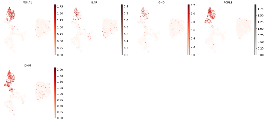

You'll notice that a single marker is often expressed across multiple clusters; truly distinguishing cell types typically requires the intersection of several markers. Furthermore, due to dropout, any given marker gene is only detected in a subset of cells. Clustering similar cells together before annotation helps compensate for these undetected transcripts.

Clustering and Visualization

We use the Leiden algorithm to cluster cells:

#sc.tl.leiden(adata, resolution=1, key_added="leiden_1")
#sc.pl.umap(adata, color="leiden_1")
# Use resolution=2 for finer cluster partitioning
sc.tl.leiden(adata, resolution=2, key_added="leiden_2")
sc.pl.umap(adata, color="leiden_2")

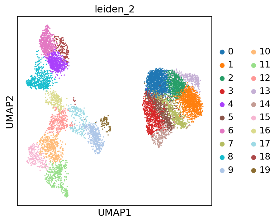
Leiden clustering at resolution 2

Use a dot plot to visualize marker gene expression across clusters:

B_plasma_markers = {
    ct: [m for m in ct_markers if m in adata.var.index]
    for ct, ct_markers in marker_genes.items()
    if ct in B_plasma_cts
}
sc.pl.dotplot(
    adata,
    groupby="leiden_2",
    var_names=B_plasma_markers,
    standard_scale="var",
)

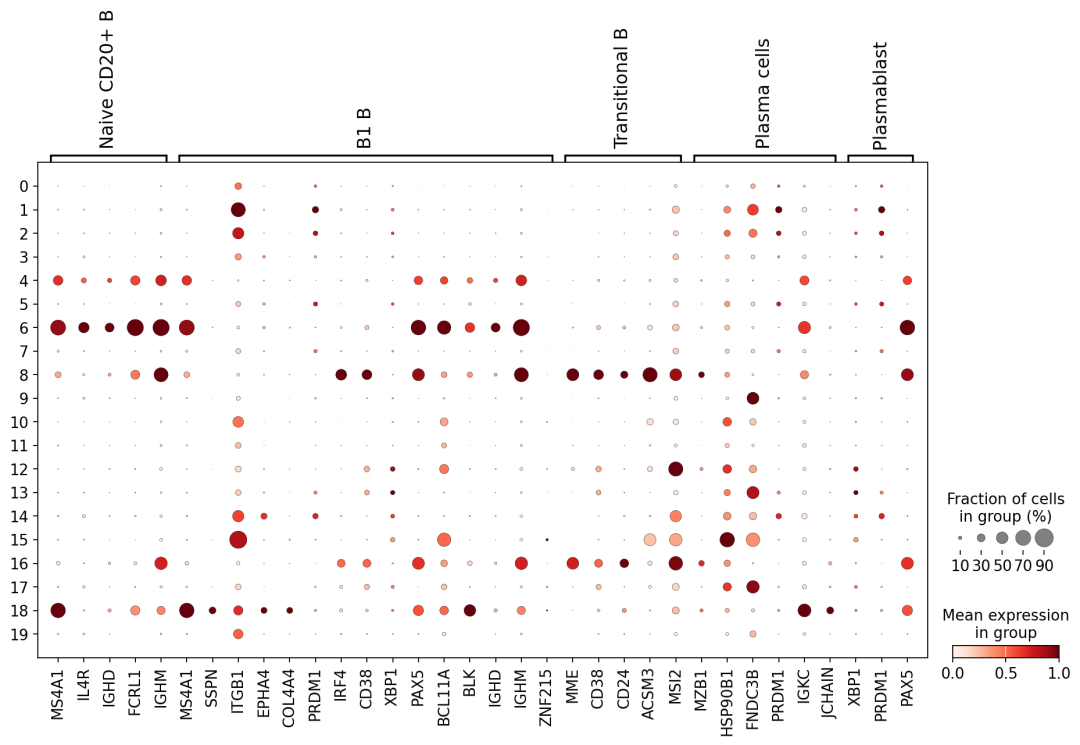
Dot plot of B/plasma cell marker genes across Leiden clusters

Based on this, we can annotate a subset of clusters:

cl_annotation = {
    "4": "Naive CD20+ B",
    "6": "Naive CD20+ B",
    "8": "Transitional B",
    "18": "B1 B",  # Note: B1 B negative markers IGHD and IGHM show lower expression here
}

adata.obs["manual_celltype_annotation"] = adata.obs.leiden_2.map(cl_annotation)

sc.pl.umap(adata, color=["manual_celltype_annotation"])

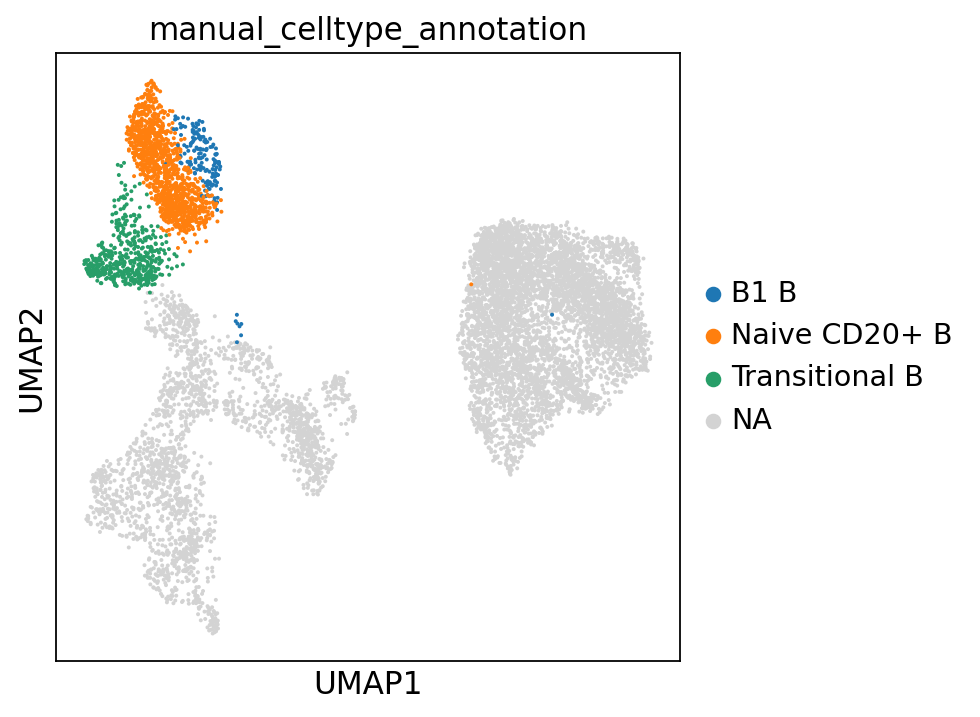
Manual annotation results on UMAP

The B1 B marker signal turns out to be diffuse — no single cluster cleanly captures this population, illustrating how marker behavior can vary considerably across datasets. This is one of the most common pitfalls of manual annotation.

Differentially Expressed Genes

The alternative approach is to first compute differentially expressed genes (DEGs) for each cluster, then cross-reference those genes against known cell type signatures.

# Compute DEGs per cluster using Wilcoxon rank-sum test
sc.tl.rank_genes_groups(
    adata, groupby="leiden_2", method="wilcoxon", key_added="dea_leiden_2"
)

# Filter for more cluster-specific genes
sc.tl.filter_rank_genes_groups(
    adata,
    min_in_group_fraction=0.2,
    max_out_group_fraction=0.2,
    key="dea_leiden_2",
    key_added="dea_leiden_2_filtered",
)

# Visualize
sc.pl.rank_genes_groups_dotplot(
    adata,
    groupby="leiden_2",
    standard_scale="var",
    n_genes=5,
    key="dea_leiden_2_filtered",
)

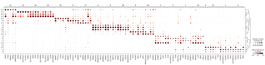
Dot plot visualization of top differentially expressed genes

Cluster 12 displays several relatively distinctive genes: CDK6, ETV6, NKAIN2, and GNAQ. A literature search reveals that NKAIN2 and ETV6 are markers of hematopoietic stem cells (HSCs). At the same time, known markers for MK/E progenitors are also expressed in cluster 12:

sc.pl.umap(
    adata,
    color=["CDK6", "ETV6", "NKAIN2", "GNAQ", "leiden_2"],
    vmax="p99",
    legend_loc="on data",
    frameon=False,
    cmap="Reds",
)
sc.pl.umap(
    adata,
    color=["ZNF385D", "ITGA2B", "RYR3", "PLCB1"],
    vmax="p99",
    legend_loc="on data",
    frameon=False,
    cmap="Reds",
)

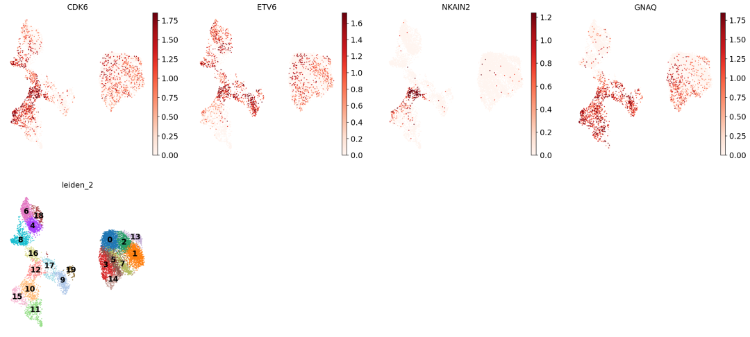
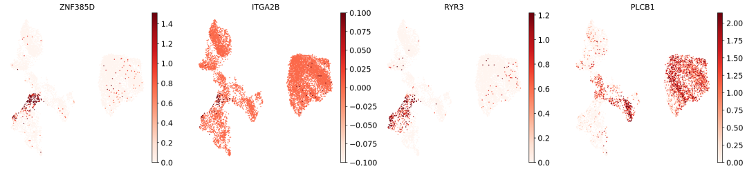
This suggests that cluster 12 is not a pure HSC population, but rather a mixed cluster of HSCs and MK/E progenitors. We can capture this uncertainty in the annotation:

cl_annotation["12"] = "HSCs + MK/E prog (?)"
adata.obs["manual_celltype_annotation"] = adata.obs.leiden_2.map(cl_annotation)

As you can see, manual annotation — while flexible and interpretable — comes with real challenges: (1) it is sensitive to marker selection, clustering resolution, and sample-to-sample variation; (2) many cell types lack unique marker genes, making it hard to determine whether a cluster is a mixed population or a novel subtype; (3) it demands substantial domain expertise. This is precisely why more and more studies are pairing manual annotation with automated tools to speed up and validate the process.

Strategy 2: Automated Annotation

Although treated as a single category here, automated annotation remains an extremely active research area. Methods based on diverse algorithms — machine learning classifiers, neural networks, large language models, and more — continue to emerge. That said, keep in mind: automated results are typically a starting point, and always require manual validation.

The quality of automated annotation depends on three key factors:

1. Classifier type: Studies have shown that different algorithms (SVM, logistic regression, neural networks, etc.) tend to perform comparably; deep learning is not always the winner.
2. Training data quality: If the training set annotations are imprecise or incorrect, the model's outputs will be too — garbage in, garbage out.
3. Data similarity: If the training set was generated by Drop-seq but your query data comes from 10x Chromium snRNA-seq, annotation reliability will suffer. The same applies to cross-tissue and cross-species scenarios.

Advantages of automated annotation:

• Fast and convenient; often no need to download and preprocess large reference datasets
• Not reliant on clustering; can operate at the single-cell level
• Leverages existing high-quality reference annotations
• Promotes consistent nomenclature across studies

A word of caution: some automated tools (particularly ML-based ones) lack transparency, so confidence/uncertainty scores should always be consulted.

CellTypist

CellTypist is a machine-learning-based automated annotation tool that uses pretrained models to predict cell types:

# Prepare data: normalize to 10,000 counts per cell, then log1p-transform
adata_celltypist = adata.copy()
adata_celltypist.X = adata.layers["counts"]
sc.pp.normalize_per_cell(adata_celltypist, counts_per_cell_after=10**4)
sc.pp.log1p(adata_celltypist)
adata_celltypist.X = adata_celltypist.X.toarray()

# Download immune cell models
models.download_models(
    force_update=True, model=["Immune_All_Low.pkl", "Immune_All_High.pkl"]
)

# Load the fine-grained model
model_low = models.Model.load(model="Immune_All_Low.pkl")
#model_high = models.Model.load(model="Immune_All_High.pkl")

# Run annotation
predictions_low = celltypist.annotate(
    adata_celltypist, model=model_low, majority_voting=True
)

# Transfer results back to the original AnnData object
predictions_low_adata = predictions_low.to_adata()
adata.obs["celltypist_cell_label_fine"] = predictions_low_adata.obs.loc[
    adata.obs.index, "majority_voting"
]
adata.obs["celltypist_conf_score_fine"] = predictions_low_adata.obs.loc[
    adata.obs.index, "conf_score"
]

Visualize the results and assess annotation quality:

sc.pl.umap(
    adata,
    color=["celltypist_cell_label_fine", "celltypist_conf_score_fine"],
    frameon=False,
)
sc.pl.dendrogram(adata, groupby="celltypist_cell_label_fine")

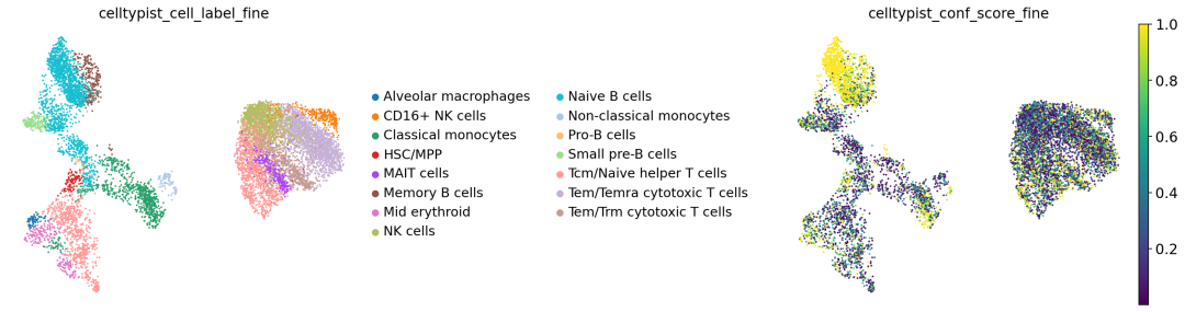
Fine-grained CellTypist annotation results and per-cell confidence scores

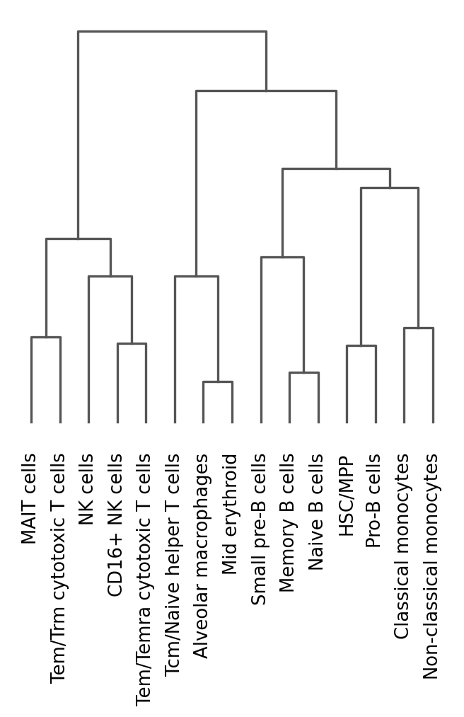
Hierarchical dendrogram of annotated cell types

The coarse-grained model follows an analogous workflow and is not repeated here for brevity.

Examining the dendrogram alongside the manual annotation comparison reveals some questionable assignments: for instance, Tcm/Naive helper T cells appear closer to erythroid cells and macrophages than to other T cell subpopulations — a red flag suggesting potential misannotation.

We can also cross-tabulate cluster 12 with CellTypist labels (sorted by frequency):

pd.crosstab(adata.obs.leiden_2, adata.obs.celltypist_cell_label_fine).loc[
    "12", :
].sort_values(ascending=False)

celltypist_cell_label_fine
Naive B cells                  98
HSC/MPP                        97
Classical monocytes            56
Pro-B cells                    28
Tcm/Naive helper T cells       13
Tem/Temra cytotoxic T cells     1
...
Name: 12, dtype: int64

This confirms the heterogeneity we suspected within cluster 12. Automated annotation results should never be accepted uncritically — careful inspection is always warranted.

scArches

This approach mirrors the logic of aligning sequencing reads to a reference genome: new query data are mapped onto a pre-annotated reference dataset, and cell type labels are transferred via k-nearest neighbor (KNN) label transfer.

★

Note: scArches leverages GPU acceleration. If your machine does not have a dedicated GPU, performance may be substantially slower or the model may not run at all.

# Prepare query data
adata_to_map = adata.copy()
adata_to_map.X = adata_to_map.layers["counts"]

# Load the gene features used by the reference model
reference_model_features = pd.read_csv(
    "https://figshare.com/ndownloader/files/41436645", index_col=0
)

# Reindex by Ensembl gene IDs to match the reference
adata_to_map.var["gene_names"] = adata_to_map.var.index
adata_to_map.var.set_index("gene_ids", inplace=True)

# Pad missing genes with zeros
missing_genes = [
    gene_id for gene_id in reference_model_features.index
    if gene_id not in adata_to_map.var.index
]

missing_gene_adata = sc.AnnData(
    X=csr_matrix(np.zeros(shape=(adata.n_obs, len(missing_genes))), dtype="float32"),
    obs=adata.obs.iloc[:, :1],
    var=reference_model_features.loc[missing_genes, :],
)

# Concatenate query data with padded missing genes
adata_to_map_augmented = sc.concat(
    [adata_to_map, missing_gene_adata], axis=1
)

Next, train the mapping model (query-to-reference):

# Load the pretrained reference model and attach query data
scarches_model = sca.models.SCVI.load_query_data(
    adata=adata_to_map_augmented,
    reference_model="./reference_model",
    freeze_dropout=True,
)

# Train the query mapping (fine-tuning)
scarches_model.train(max_epochs=500, plan_kwargs=dict(weight_decay=0.0))

# Extract the latent embedding for query cells
adata.obsm["X_scVI"] = scarches_model.get_latent_representation()

Quickly visualize the new embedding to confirm that known cell types remain coherently grouped:

sc.pp.neighbors(adata, use_rep="X_scVI")
sc.tl.umap(adata)
sc.pl.umap(
    adata,
    color=["IGHD", "IGHM", "PRDM1"],
    vmin=0,
    vmax="p99",
    sort_order=False,
    frameon=False,
    cmap="Reds"
)

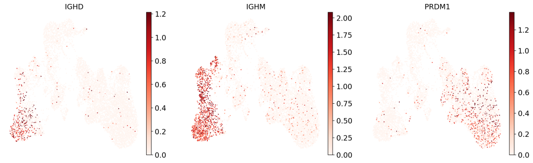
Now perform KNN-based label transfer from the reference embedding:

# Load the reference embedding
ref_emb = sc.read(
    filename="reference_embedding.h5ad",
    backup_url="https://figshare.com/ndownloader/files/41376264",
)

# Create an AnnData object for the query embedding
adata_emb = sc.AnnData(X=adata.obsm["X_scVI"], obs=adata.obs)

# Concatenate reference and query embeddings
emb_ref_query = sc.concat([ref_emb, adata_emb], axis=0)

# Train the weighted KNN model on the reference
knn_transformer = sca.utils.knn.weighted_knn_trainer(
    train_adata=ref_emb,
    train_adata_emb="X",
    n_neighbors=15,
)

# Transfer labels from reference to query
labels, uncert = sca.utils.knn.weighted_knn_transfer(
    query_adata=adata_emb,
    query_adata_emb="X",
    label_keys="cell_type",
    knn_model=knn_transformer,
    ref_adata_obs=ref_emb.obs,
)

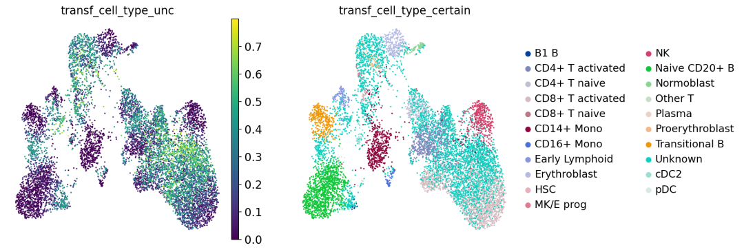
Inspect the transferred annotations, flagging high-uncertainty cells:

# Label cells with high uncertainty as "Unknown"
adata.obs["transf_cell_type_certain"] = adata.obs.transf_cell_type.tolist()
adata.obs.loc[
    adata.obs.transf_cell_type_unc > 0.2, "transf_cell_type_certain"
] = "Unknown"

sc.pl.umap(adata, color="transf_cell_type_certain", frameon=False)

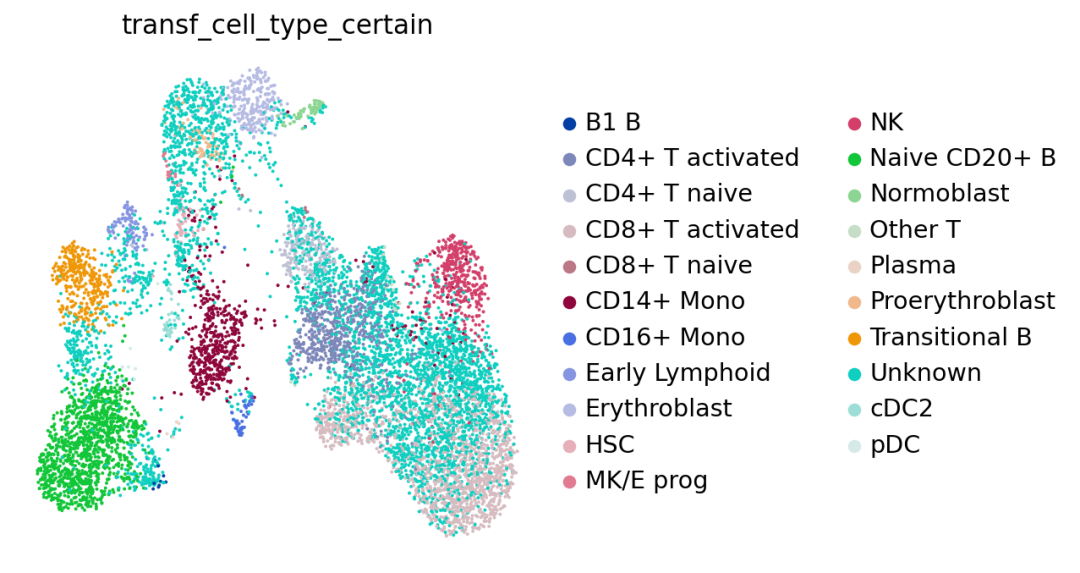
A substantial number of cells are labeled "Unknown," indicating they require further manual inspection.

Let's validate the transferred labels by checking known marker gene expression:

# Verify marker expression for selected cell types
cell_types_to_check = [
    "CD14+ Mono", "cDC2", "NK", "B1 B",
    "CD4+ T activated", "T naive", "MK/E prog",
]

sc.pl.dotplot(
    adata,
    var_names={ct: marker_genes_in_data[ct] for ct in cell_types_to_check},
    groupby="transf_cell_type_certain",
    standard_scale="var",
)

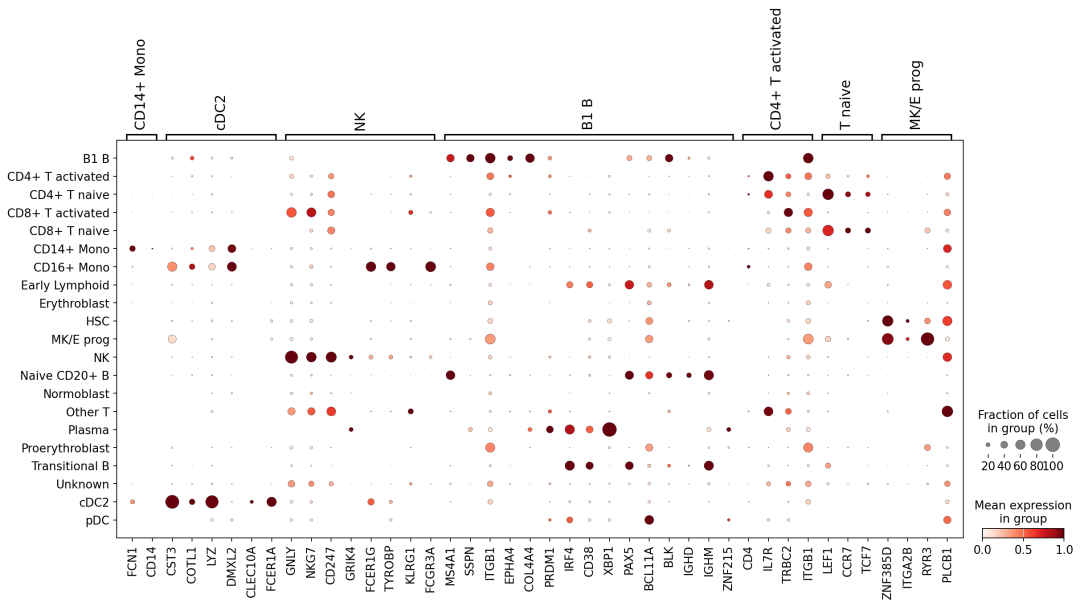
Finally, visualize annotation uncertainty to identify regions that warrant closer attention:

sc.pl.umap(
    adata, color=["transf_cell_type_unc", "transf_cell_type_certain"], frameon=False
)

Save the intermediate results:

# adata.write("./annotation_adata_out.h5ad")

Closing Thoughts

Cell annotation is one of the most critical — and most challenging — steps in single-cell analysis. Accurate cell type identification underpins the reliability of everything that follows: identifying disease-associated cell subpopulations, tracing developmental trajectories, and studying cell–cell communication.

Current Challenges

• Lack of standardization: Different studies adopt different cell type nomenclatures, with no widely accepted unified standard
• Resolution dilemma: How granular should you go? CD4+ T cells? Or Th1/Th2/Th17?
• Continuity vs. discreteness: Many cells exist along a continuous spectrum; forcing discrete labels may obscure biologically meaningful transitions
• Batch effects: Technical variation across experimental conditions and sequencing platforms can mask true biological signals

Recent Advances

• Large-scale reference atlases: Projects such as the Human Cell Atlas and CZI CELLxGENE are building comprehensive reference maps of all human cell types
• Foundation models: Large pretrained models like scGPT and Geneformer are being applied to cell annotation, enabling handling of increasingly complex scenarios
• Multimodal integration: Combining transcriptomics, proteomics, epigenomics, and other data modalities for richer, more accurate annotation
• Uncertainty quantification: A growing number of tools provide per-cell confidence scores to flag regions requiring manual review
• Hierarchical annotation: Multi-resolution annotation frameworks, from coarse to fine, tailored to different research questions

Practical Recommendations

For cell annotation in real-world projects, a multi-pronged strategy is recommended:

1. Use automated tools to obtain a quick initial annotation
2. Compare results across multiple tools and prioritize high-consensus labels
3. Validate key cell type assignments against known marker gene expression
4. Retain uncertainty scores, and manually review low-confidence regions
5. Collaborate with domain experts to ensure biologically sound interpretations

We've also published several annotation-focused articles on our WeChat channel — check them out: I'd call the new Azimuth the best annotation tool out there, and a piece on using LLMs to assist with marker gene retrieval via GPTcelltype: The Future Is Now: The Era of LLM × Single-Cell Has Begun

---

Originally posted on WeChat Official Account: bioinfo_studyroom