Single-Cell Analysis with Theis Lab: Alignment and Mapping Done Right

February 20, 2026 · 14 min read · Tutorials

Cracking single-cell analysis with Theis Lab

No.04 | Published: 2025-01-22 | Estimated read time: 17 minutes

Single-Cell Best Practices

Sequence Alignment and Mapping

In this section:

Introduction to commonly used alignment tools
Genome-level vs. transcriptome-level mapping
Choosing a reference sequence

Sequence Mapping/Alignment is the foundational step in processing raw single-cell data. Its core goal is to determine the likely origin of each sequenced fragment within the genome or transcriptome — in other words, to find the region of the reference sequence that best matches each sequencing read.

Depending on the sequencing protocol, raw sequencing files may contain the following information:

Cell Barcodes (CB): used to label individual cells
Unique Molecular Identifiers (UMI): used to distinguish individual RNA molecules
cDNA reads: the sequencing output from RNA molecules

As the first step in single-cell data processing (Figure 3.1), accurate alignment is critical. If reads are incorrectly mapped to genes or transcripts, all downstream analyses — such as generating a gene expression matrix — will also produce incorrect or misleading results.

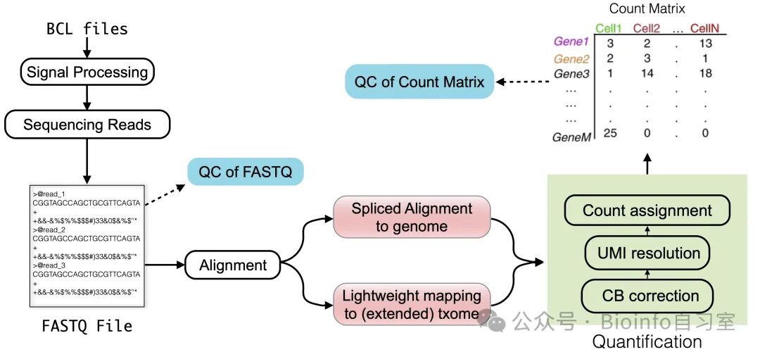
Figure 1. The full upstream analysis workflow for sequencing data — also the roadmap for this chapter. You've seen it before in the previous post — do you remember it?

Technical Challenges and Specialized Tools

While sequence alignment technology predates single-cell RNA sequencing (scRNA-seq), the sheer scale of single-cell data — typically hundreds of millions to billions of reads — demands enormous computational resources. Moreover, applying conventional bulk RNA-seq alignment tools directly leads to several problems, since these tools are not designed with single-cell protocols in mind:

Additional tools are needed to handle single-cell-specific information (e.g., the positions of cell barcodes and UMIs)
Sample demultiplexing and UMI resolution must be performed as separate steps
Large numbers of intermediate files are generated, significantly increasing storage requirements and I/O overhead

To address these issues, researchers have developed alignment tools specifically designed for scRNA-seq. These tools handle the unique requirements of single-cell data automatically. They include 10x Genomics' commercial software Cell Ranger, as well as open-source alternatives: zUMIs, alevin, RainDrop, kallisto|bustools, STARsolo, alevin-fry, and others. All of these provide user-friendly interfaces and integrate technical sequence parsing (CB/UMI processing), demultiplexing, and UMI resolution into a single workflow. Some tools also employ strategies that minimize or eliminate intermediate files to cope with the large data volumes and computational burden.

Although different alignment tools differ substantially in their algorithms, data structures, and computational trade-offs, they can be categorized along two dimensions: the type of alignment algorithm and the type of reference sequence.

3.2.1 Types of Alignment Algorithms

In single-cell and single-nucleus RNA sequencing (sc/snRNA-seq), commonly used alignment algorithms fall into three categories: spliced alignment, contiguous alignment, and variants of lightweight mapping. As illustrated in Figure 3.14, we broadly divide methods into two camps: "alignment-based" and "lightweight mapping-based."

Alignment-based methods first use a series of heuristics to identify candidate locations in the reference genome or transcriptome where a read might originate, and then perform a more detailed nucleotide-level alignment and scoring at each candidate site. This process typically relies on dynamic programming (DP) algorithms. By contrast, lightweight mapping methods skip nucleotide-level comparison entirely. Instead, they use pattern matching based on k-mers or similar exact-match rules to rapidly infer the likely mapping locations of each read, achieving substantially higher speed and throughput.

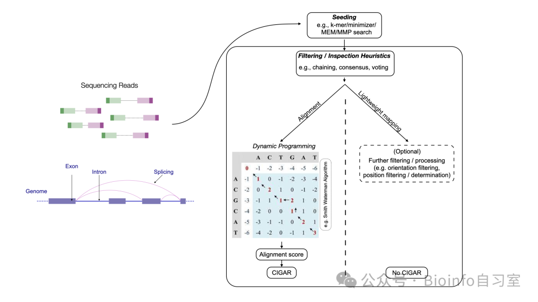
Figure 2. Overview of alignment-based vs. mapping-based methods. One key distinction: alignment-based methods produce an "alignment score," while mapping-based methods do not.

Dynamic Programming Algorithms

Dynamic programming (DP) has a long and rich history as the backbone of sequence alignment. Depending on the requirements, alignments can be classified as follows:

Global alignment: requires all bases of both the read and the reference to be aligned end-to-end.
Local alignment: finds the optimal match within a subsequence of either the read or the reference.
Semi-global alignment (also called "fitting" alignment): typically used for short-read sequencing. It assumes that most of the read aligns to some substring of the reference, while allowing mismatches or gaps at the ends of the read or the reference.
Extension alignment: applies lower penalties (i.e., "soft clipping") for insertions, deletions, or mismatches at the ends of a read, effectively ignoring or down-weighting poor-quality bases at the read edges.

All of these methods fundamentally rely on a DP table. Their time complexity is comparable to classical dynamic programming, but can be improved substantially through various optimization techniques.

Alignment and Dynamic Programming — A Closer Look

Dynamic programming works by breaking a complex, large problem into many smaller, related subproblems, solving each one, and then combining the solutions to arrive at the answer to the original problem. The core idea is:

Decompose: split the problem into interrelated subproblems according to a defined rule;

Store: record or cache the solution to each subproblem;

Combine: when a larger subproblem (or the full problem) needs the result of a previous subproblem, simply look it up rather than recomputing it.

This approach eliminates redundant computation and dramatically improves efficiency.

Sequence alignment can be thought of as a "shortest path" or "minimum cost" problem:

Given two sequences (e.g., a genomic reference and a sequencing read), we want to find the best way to match them.

The matching process follows a scoring scheme — for example, matching bases earn points; mismatches are penalized; insertions or deletions (indels) are also penalized.

To find the globally optimal alignment (highest score / lowest cost), we need to explore different alignment configurations. Exhaustive enumeration would be computationally prohibitive.

Dynamic programming elegantly solves this:

It breaks the alignment into smaller subproblems, comparing one base at a time against the corresponding reference position;

Each cell in the "alignment matrix" stores the best alignment score for a subproblem, which in turn depends on previously computed scores in adjacent cells;

Once the full alignment matrix is filled, we can read the overall optimal alignment score and traceback path from the bottom-right corner (or another terminal position of the matrix).

This design perfectly suits the dynamic programming paradigm: overlapping subproblems (comparing each base to its reference counterpart at every step), incrementally accumulated and reused results (the scores from the cell above, to the left, or diagonally above-left feed into the current cell's computation).

In the context of genomic alignment, many algorithms incorporate advanced optimizations and heuristics to improve efficiency and practical applicability:

Banded alignment: if users do not care about alignment scores below a certain threshold, a large number of DP cells can be skipped.
X-drop and Z-drop: enable early "pruning," discarding alignment paths that are unlikely to yield high scores.
Wavefront alignment: when a high-scoring (low-divergence) alignment exists, this approach can drastically reduce both the theoretical and practical time and memory requirements.
Data layout and parallel computation optimizations, including restructuring the DP computation for SIMD vectorization (i.e., applying the same instruction to multiple data elements simultaneously).

Most widely used alignment tools today integrate these highly optimized and parallelized methods, resulting in dramatically reduced runtimes.

Alignment Scores and Alignment Paths (CIGAR Strings)

Along with the alignment score, we can also traceback the actual alignment path that produced the score. This information is typically stored in output SAM/BAM files as a CIGAR string (Concise Idiosyncratic Gapped Alignment Report).

Decoding CIGAR Strings

A standard CIGAR string uses the following characters:

M: Match or Mismatch

I: Insertion (relative to the reference)

D: Deletion (relative to the reference)

N: Skipped region (typically represents an intron)

S: Soft Clipping (part of the read is unaligned but retained in the data)

H: Hard Clipping (part of the read is unaligned and removed from the data)

P: Padding (alignment gap inserted in the reference)

For example: 3M2D4M means the first 3 bases are matches/mismatches (M), followed by a 2-base deletion (D, present in the reference but absent in the read), then 4 more matches/mismatches.

Extended CIGAR distinguishes between matches and mismatches:

=: Match

X: Mismatch

For example: 3=2D2=2X means 3 exact matches, a 2-base deletion, 2 more matches, then 2 mismatches.

Alignment-based methods not only compute alignment scores, but also assess whether each read is a "high-quality" match to the reference — helping to filter out erroneous mappings caused by low-complexity sequences or spurious hits.

Full-alignment tools (e.g., STAR, STARsolo): perform the complete DP traceback and report the full alignment path.
Selective alignment (e.g., Salmon, alevin): evaluate alignment scores but skip the detailed traceback of the optimal path, reducing computational overhead.

Spliced Alignment vs. Contiguous Alignment

As mentioned above, alignment-based methods can be further divided into spliced and contiguous alignment (lightweight mapping methods currently cannot achieve full alignment).

Spliced alignment: aligns a read in multiple segments to the reference genome/transcriptome, allowing two adjacent segments of the read to map to positions that are far apart in the reference (e.g., spanning an intron or a large insertion). This is critically important for RNA-seq reads aligned to the genome, because transcripts may span one or more splice junctions — a read may be continuous in the transcript, but its sequence is distributed across different exons and introns in the genome. The challenge of spliced alignment lies in accurately localizing a short read segment that crosses a splice junction using very limited information.
Contiguous alignment: assumes that a read aligns to a single contiguous stretch of the reference. Small indels are permitted, but there are no multi-kilobase gaps like those seen in spliced alignment.

Lightweight Mapping Methods

Finally, let's revisit lightweight mapping — the alternative to alignment-based approaches. Representative algorithms include pseudoalignment, quasi-mapping, and structural-constraint pseudoalignment.

As described above, these methods skip nucleotide-by-nucleotide comparison. Instead, they rapidly infer the likely mapping location of a read based on the distribution, orientation, and relative positions of a set of matching k-mers (or other exact-match patterns). This dramatically outperforms alignment-based methods in speed and throughput. However, because nucleotide-level alignment information is absent, it is difficult to obtain score-based quality assessments, making it harder to judge whether the match between a read and the reference is of sufficient confidence.

In summary:

Alignment-based methods provide richer quality scores and alignment details; they are best suited for analyses requiring fine-grained precision.
Lightweight mapping methods emphasize speed and throughput; they are ideal for large-scale workflows where nucleotide-level alignment is not critical.
For RNA-seq, particularly when alternative splicing is involved, spliced alignment is essential; when only continuous reference regions are needed, contiguous alignment tools suffice.

3.2.2 Types of Reference Sequences

Decisions in mapping don't end with the choice of algorithm — they also involve choosing the reference sequence used for mapping. We classify reference sequences into three broad categories:

The complete reference genome
An annotated transcriptome (spliced transcriptome)
An augmented transcriptome

It is worth noting that not all combinations of mapping algorithm and reference sequence are currently feasible. For example, no lightweight mapping method currently exists that can perform spliced mapping directly against a reference genome.

Mapping to the Genome

The first category uses the complete genome of the organism of interest as the reference, typically in conjunction with transcript annotations during the mapping process. Tools that use this approach include zUMIs, Cell Ranger, and STARsolo.

Because many reads originate from spliced transcripts, this approach allows split alignment of a single read across one or more splice junctions.

Advantages:

Full coverage: can handle reads from anywhere in the genome, not just annotated transcripts
Low marginal cost of index construction: once a genome-scale index is built, processing additional reads from intronic regions incurs almost no additional cost. Genome-based mapping is therefore applicable to both single-cell and single-nucleus sequencing data.
Extensibility: can reveal expression in unannotated regions, facilitating downstream discoveries (e.g., UTR extensions found by Pool et al., 2022)

Limitations:

High memory requirements: for the human genome, building and storing an index requires over 32 GB of RAM. While sparse suffix arrays can compress the index to save storage, this reduces mapping speed, and the memory required to build the initial index remains unchanged.
High computational cost: handling splice junctions and computing alignment scores requires relatively complex algorithms, imposing a heavier computational burden.
Reference availability: a reference genome must exist, which can be a challenge for non-model organisms.

Mapping to the Spliced Transcriptome

To reduce the computational overhead of genome-wide spliced alignment, a widely adopted alternative is to use only the sequences of annotated transcripts as the reference. Since most single-cell experiments involve model organisms with well-annotated transcriptomes (e.g., mouse or human), transcriptome-based quantification typically achieves similar read coverage to genome-based approaches.

Advantages of this approach:

Smaller reference: the transcriptome is much smaller than the full genome, reducing the computational resources required for mapping.
Simplified alignment: splicing patterns are already encoded in the transcript sequences, so there is no need to solve the complex spliced alignment problem — only contiguous alignment or mapping is required.
Compatibility with multiple methods: since only contiguous alignments need to be found, this approach is compatible with both traditional alignment algorithms and lightweight mapping techniques. Many popular tools target the spliced transcriptome for exactly this reason.

However, this approach has notable limitations:

Cannot capture reads from outside the spliced transcriptome: this makes the approach unsuitable for single-nucleus sequencing data. Even in single-cell experiments, reads originating outside the spliced transcriptome can constitute a substantial fraction, and growing evidence suggests these reads may contain important biological information that should be incorporated into downstream analyses.
Potential for misalignment: when combined with lightweight mapping methods, short matches between the spliced transcriptome and reads that truly originate elsewhere can produce false positives, leading to incorrect or even biologically implausible gene expression estimates.

Mapping to the Augmented Transcriptome

To address the problem of reads originating from regions outside the spliced transcriptome, researchers developed the augmented transcriptome approach. This involves supplementing the spliced transcript sequences with additional reference sequences from which reads may originate — such as fully unspliced transcripts or excised intron sequences.

Key features and advantages:

Smaller index size compared to the full genome
Still only requires searching for contiguous read alignments
Faster mapping with lower memory requirements
Can capture reads from outside the spliced transcriptome
Significantly reduces false-positive mappings when using lightweight mapping methods
Widely used in single-nucleus sequencing data analysis and RNA velocity analysis
Compatible with most analysis approaches that do not require spliced alignment to the full genome

This approach is valuable even for standard single-cell RNA-seq data. A commonly constructed augmented transcriptome is known as splici (short for spliced + intronic). The splici reference consists of the spliced transcriptome sequences combined with the merged interval sequences of annotated gene introns; each reference sequence is labeled according to its annotated splicing status.

The key advantages of this strategy are: (1) it allows the use of lightweight mapping while substantially reducing misalignment; (2) it simultaneously captures reads from both spliced and unspliced origins, improving the sensitivity of downstream analyses. Furthermore, because splicing status is tracked and reported separately during quantification, this approach unifies preprocessing for single-cell, single-nucleus, and RNA dynamics workflows — striking a balance between speed and accuracy, and making it particularly well-suited for studies that need to consider multiple RNA forms simultaneously.

Closing Notes

This post again draws from the intensely technical Chapter 3 of the original book, walking you through the algorithms underlying alignment and mapping of sequencing data. The remaining material can be broken into roughly 3–4 more parts, covering topics such as cell barcode and UMI processing, count matrix generation and quality control, and hands-on alevin-fry code walkthroughs. We'll release the access code and supplementary materials all at once once everything is compiled — stay tuned!

Next up: Cell Barcode and UMI Processing. Don't miss it!

Previous in-depth single-cell tutorials ⬇️ — you'll never be left wondering why again:

Single-Cell Analysis with Theis Lab: Overview of Single-Cell Sequencing · 2024-12-16

Single-Cell Analysis with Theis Lab: How to Read a QC Report · 2025-01-17

Forward · Bookmark · Like · In Reading

Originally posted on WeChat Official Account: bioinfo_studyroom

Single Cell Tutorial