SCIPAC: Discovering Clinically Relevant Cell Populations in Single-Cell Data

Today I'd like to introduce a truly gem of an R package — SCIPAC. Published in 2024 in the prestigious journal Genome Biology, SCIPAC is designed to quantitatively assess the association strength between individual cells and clinical phenotypes in single-cell data. In plain terms, it helps you identify the "star cell populations" most relevant to a disease of interest.
🔍 Why Do We Need SCIPAC?
The Limitations of Traditional Approaches
Suppose you have a breast cancer single-cell dataset and have identified several T cell subpopulations. You want to know: which T cells are genuinely associated with tumor malignancy? Which ones are bystanders?
Traditional single-cell analysis can tell you cell types, but it cannot quantify their relationship to clinical phenotypes. A common workaround is to export marker gene sets for each subpopulation and perform correlation analysis in a public database. However, this approach has serious flaws:
- Gene expression ≠ Cell proportion: High expression of a gene in TCGA does not necessarily mean that cells expressing that gene are abundant in the tumor. A cell type may have low per-cell expression but be numerically dominant; another may show high expression levels but be extremely rare.
- Severe batch effects: Single-cell and bulk RNA-seq data originate from different experimental platforms and processing pipelines. Direct comparison is prone to generating false positives.
- No statistical framework: This kind of ad hoc analysis lacks rigorous statistical grounding and cannot provide p-values or confidence intervals.
- Labor-intensive: Each cell type must be analyzed separately with manually curated gene sets — an inefficient and error-prone process.
The earlier and more widely known Scissor method (Sun et al., Nat Biotech 2021) was pioneering in proposing a joint single-cell/bulk data analysis framework, but it can only classify cells into three coarse categories — "positively correlated," "negatively correlated," and "unrelated" — with no quantitative information:
- 🔴 Scissor+ cells: Positively correlated with the phenotype — but how strong is the association?
- 🔵 Scissor− cells: Negatively correlated with the phenotype — but what is the magnitude of the effect?
- ⚪ Background cells: Truly unrelated? Or just a weak association below the detection threshold?
Furthermore, Scissor's results are highly sensitive to the choice of the regularization parameter α. Different values of α can yield completely different outcomes, with no objective criterion for selecting the optimal setting. Researchers are often forced to try multiple parameter values and pick whichever result "looks reasonable" — which is hardly rigorous.
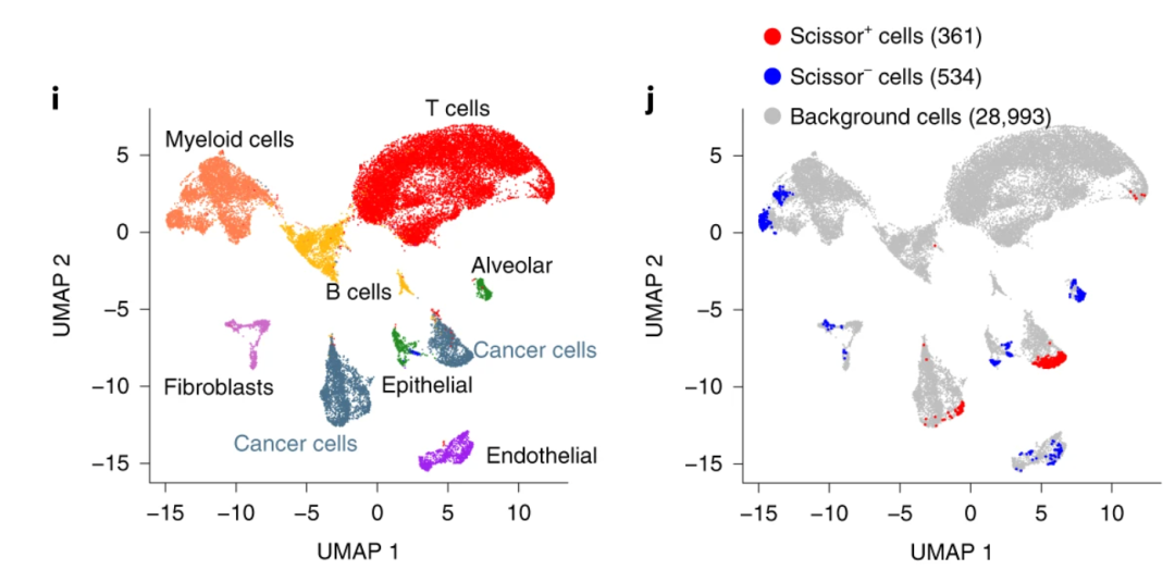 Scissor example. Sun et al., Nat Biotech 2021
This is the core problem SCIPAC was designed to solve: not only identifying which cells are associated with disease, but precisely quantifying the strength of that association and providing formal statistical significance testing.
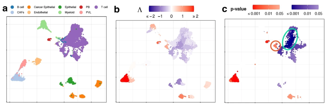 SCIPAC example. Gan et al., Genome Biol 2024
What Makes SCIPAC Innovative
SCIPAC's core idea is elegantly simple: If an increase in the proportion of a particular cell type raises the probability of disease occurrence, then that cell type is positively associated with the disease.
Its key advantages include:
- Quantitative assessment: Reports a specific association strength value (the λ statistic)
- Statistical significance: Provides a p-value for every association
- Multiple phenotype types supported: Binary classification, continuous variables, survival data, and ordinal categories
- Computationally efficient: Dozens of times faster than Scissor
- Minimal parameter tuning: Works well with default settings in most cases
- Seurat integration: Fits seamlessly into standard single-cell analysis workflows
Hands-On Tutorial: GSE176078 Breast Cancer Dataset
Let's walk through a complete SCIPAC analysis using a real-world dataset.
 Wu et al., Nat Genet 2021
This breast cancer single-cell dataset contains 26 samples spanning three molecular subtypes — HER2+, ER+, and TNBC — and is available for download at GSE176078.
What You'll Need
- An annotated Seurat object
obj(or a raw count matrix with cell annotations). Format: genes as rows, cell barcodes as columns. - A bulk RNA-seq expression matrix with matched clinical information. Normalized formats (TPM/RPKM/FPKM/RSEM) are preferred, but raw counts can be normalized manually. Format: genes as rows, sample IDs as columns.
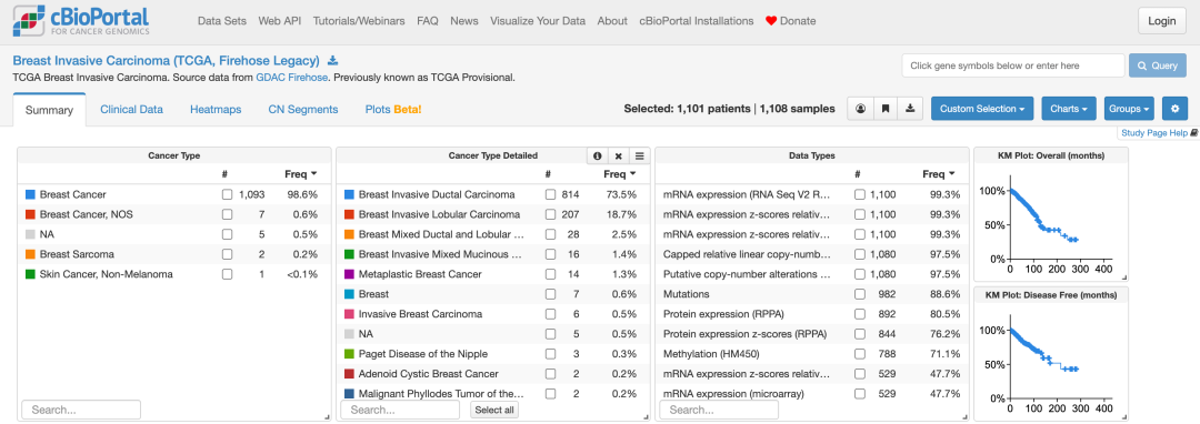 TCGA_BRCA (firehose legacy)
Install and load the required R packages:
devtools::install_github('RavenGan/SCIPAC')
library(Seurat)
library(SCIPAC)
library(tidyverse)
Process the bulk data (RSEM is already normalized, so no further normalization is needed):
# Expression matrix — remember to replace with your actual file path
tcga_expr <- read.delim("brca_tcga/data_mrna_seq_v2_rsem.txt", comment.char="#")
# Sample-level clinical information
tcga_sample <- read.delim("brca_tcga/data_clinical_sample.txt", comment.char="#")
# Patient-level clinical information
tcga_patient <- read.delim("brca_tcga/data_clinical_patient.txt", comment.char="#")
# Merge sample and patient metadata
tcga_meta <- left_join(tcga_sample, tcga_patient, by="PATIENT_ID")

# Data cleaning — adjust as needed for your data
# Set gene symbols as row names (aggregate duplicate symbols by summing)
tcga_expr <- tcga_expr %>% aggregate(. ~ Hugo_Symbol, FUN=sum) %>%
  select(-Entrez_Gene_Id) %>%
  column_to_rownames("Hugo_Symbol")

# Harmonize sample ID format between metadata and expression matrix
tcga_meta$SAMPLE_ID <- gsub("-", "\\.", tcga_meta$SAMPLE_ID)

# Ensure clinical metadata and RNA-seq samples are in matching order
tcga_meta <- tcga_meta %>%
  filter(SAMPLE_ID %in% colnames(tcga_expr)) %>%
  arrange(match(SAMPLE_ID, colnames(tcga_expr)))
# Sanity check — should return TRUE
all(tcga_meta$SAMPLE_ID == colnames(tcga_expr))

# Replace placeholder strings with NA
tcga_meta[tcga_meta == "[Not Available]"] <- NA
tcga_meta[tcga_meta == "[Not Applicable]"] <- NA
# Check which clinical variables contain missing values
colSums(is.na(tcga_meta))

dim(tcga_expr) # 20513  1100
dim(tcga_meta) # 1100  137
Next, load the single-cell data. We only need the raw count matrix here (which can also be extracted from an existing Seurat object via obj[["RNA"]]$counts). Conveniently, the original publication also provides pre-computed cell type annotations.
data.path <- "~/Downloads/GSE176078_RAW/"
# Read the raw count matrix
dat <- ReadMtx(mtx=paste0(data.path, "count_matrix_sparse.mtx"),
               cells = paste0(data.path, "count_matrix_barcodes.tsv"),
               features=paste0(data.path, "count_matrix_genes.tsv"), feature.column = 1)
meta <- read.csv(paste0(data.path, "metadata.csv"))
obj <- CreateSeuratObject(dat, meta.data = meta)

# Standard preprocessing pipeline — simplified here for tutorial purposes!
obj <- NormalizeData(obj) %>%
  FindVariableFeatures() %>%
  ScaleData() %>%
  RunPCA() %>%
  RunUMAP(dims = 1:30) %>%
  FindNeighbors(dims = 1:30) %>%
  FindClusters(resolution = 0.5)
obj
An object of class Seurat
29733 features across 100064 samples within 1 assay
Active assay: RNA (29733 features, 2000 variable features)
 3 layers present: counts, data, scale.data
 2 dimensional reductions calculated: pca, umap
SCIPAC: Preprocessing
With both single-cell and bulk datasets in hand, we're ready to run SCIPAC. The first step is selecting a set of shared highly variable genes (HVGs; 1,000 by default):
# Use the raw count matrix `dat` directly as SCIPAC input
# Alternatively, extract it from an existing Seurat object:
dat <- obj[["RNA"]]$counts

# Preprocessing: find shared HVGs and subset both datasets
sc.bulk.prec <- preprocess.sc.bulk.dat(dat, tcga_expr, hvg = 1000)
# Returns a list containing the preprocessed single-cell and bulk matrices
# Both matrices will share the same 1,000 genes after processing
sc.dat.prep <- sc.bulk.prec$sc.dat.preprocessed
bulk.dat.prep <- sc.bulk.prec$bulk.dat.preprocessed
dim(sc.dat.prep)  # 1000 99664
dim(bulk.dat.prep) # 1000 1100
all(rownames(sc.dat.prep)==rownames(bulk.dat.prep)) # TRUE
The preprocess.sc.bulk.dat function does the following:
- Identifies genes present in both the single-cell and bulk datasets
- Selects the top 1,000 highly variable genes from the single-cell data within that overlap
- Subsets both matrices to those genes
By restricting all downstream steps to this gene subset, computation is greatly accelerated — making it tractable even for datasets with hundreds of thousands of cells. If you need higher accuracy, simply increase the hvg parameter.
SCIPAC: Joint PCA Dimensionality Reduction
The next step is joint PCA to project both datasets into a shared feature space.
# Default: 60 PCs; adjust as needed
pca.res <- sc.bulk.pca(sc.dat.prep, bulk.dat.prep, do.pca.sc = FALSE, n.pc = 60)

# Extract the dimensionality-reduced matrices
sc.dat.dim.redu <- pca.res$sc.dat.rot
bulk.dat.dim.redu <- pca.res$bulk.dat.rot

# Check dimensions
dim(sc.dat.dim.redu)   # 99664  60
dim(bulk.dat.dim.redu) # 1100   60
The sc.bulk.pca function performs two operations:
- Runs PCA on the bulk data
- Projects the single-cell data onto the bulk PCA rotation matrix
The key intuition is to use the principal component axes derived from bulk data to transform the single-cell data. Setting do.pca.sc = TRUE reverses this: PCA is first computed on the single-cell data and then applied to the bulk. Either direction is valid — the goal is to embed both datasets into the same latent space so they can be directly compared.
⚠️ Editor's note: Joint dimensionality reduction is a critical step. Because single-cell and bulk RNA-seq data have fundamentally different distributions and feature spaces, projecting them into a common latent space is what makes downstream integration meaningful. Dimensionality reduction is not limited to PCA — interested readers may also explore MDS, NMF, or other approaches.
SCIPAC: Clustering
ct.res <- seurat.ct(sc.dat.dim.redu, res = 1.5)
summary(ct.res) # Returns a list
#              Length Class      Mode
#k                1   -none-     numeric
#ct.assignment    1   data.frame list
#centers       3420   -none-     numeric
This step calls Seurat's FindNeighbors and FindClusters under the hood (other clustering methods can also be used). It returns the number of clusters k, the cluster assignment for each cell ct.assignment, and the cluster centroids centers. Phenotype associations are subsequently computed at the cluster level, so increasing res will yield finer-grained predictions.
⚠️ Editor's note: You might wonder why we don't just use the clustering results already stored in the Seurat object. The reason is that SCIPAC applies a different preprocessing pipeline from the standard Seurat workflow — including gene intersection with the bulk data, a different number of HVGs, and using the bulk PCA rotation matrix. In principle, if you start from scratch with identical genes in both datasets, match all parameters (HVGs, number of PCs, clustering resolution, etc.), and choose to project single-cell PCA coordinates onto the bulk space, you could reuse the clustering from your Seurat object directly.
SCIPAC: Predicting Phenotype-Associated Cells
With preprocessing complete, we can now select a phenotype of interest and identify the single-cell populations associated with it.
The SCIPAC main function takes three inputs:
- PCA-reduced bulk data matrix:
bulk.dat.dim.redu - Phenotype vector or matrix:
y - Single-cell clustering result:
ct.res
Important: The length of y must match the number of rows in bulk.dat.dim.redu (i.e., one entry per bulk sample). If any samples have missing phenotype values (NA), filter both y and bulk.dat.dim.redu to remove them before running.
Below, we demonstrate SCIPAC with three phenotype types: tumor recurrence status (binary), tumor stage (ordinal), and overall survival (time-to-event).
1. Tumor Recurrence Status (Binary)
The TCGA-BRCA clinical dataset includes a TUMOR_STATUS field indicating tumor recurrence.
table(tcga_meta$TUMOR_STATUS, useNA = "always")

#TUMOR FREE WITH TUMOR       <NA>
#       879         96        125

# Remove samples with missing tumor status, and subset the PCA matrix accordingly
tcga_meta.sub <- tcga_meta[!is.na(tcga_meta$TUMOR_STATUS), ]
bulk.dat.dim.redu.sub <- bulk.dat.dim.redu[rownames(bulk.dat.dim.redu) %in% tcga_meta.sub$SAMPLE_ID, ]

# Encode tumor status as a binary vector
y <- ifelse(tcga_meta.sub$TUMOR_STATUS=="WITH TUMOR", 1, 0)

# Sanity check
all(rownames(bulk.dat.dim.redu.sub) == rownames(y)) # TRUE
Run SCIPAC with family = "binomial" for binary outcomes:
SCIPAC.res <- SCIPAC(bulk.dat = bulk.dat.dim.redu.sub, y = y,
                     family = "binomial", ct.res = ct.res,
                     ela.net.alpha = 0.4, bt.size = 50,
                     numCores = 7, CI.alpha = 0.05, nfold = 10)
The function returns a six-column data frame:
| Column | Meaning | Notes |
|---|---|---|
| cluster_assignment | Cluster assignment | The cluster ID for each cell |
| Lambda.est | Association strength estimate | Quantifies cell–phenotype association; positive = positive correlation, negative = negative correlation |
| Lambda.upper / Lambda.lower | Confidence interval | Upper and lower bounds of the confidence interval for Lambda.est |
| sig | Significance label | Not.sig: not significant; Sig.pos: significantly positive; Sig.neg: significantly negative |
| log.pval | Log-transformed p-value | Signed log p-value; sign matches the direction of Lambda.est |
Lambda (λ) is the quantitative measure of cell type–phenotype association strength: it reflects the change in phenotype probability when the proportion of a given cell type increases.
Let's visualize the results:
# Add SCIPAC results to the Seurat object as metadata
obj <- AddMetaData(obj, metadata = SCIPAC.res)

library(RColorBrewer)
p1 <- DimPlot(obj, group.by = "celltype_major", label=T)
p2 <- FeaturePlot(obj, "Lambda.est", order=T) +
  scale_color_gradientn(colours = rev(brewer.pal(11, "RdBu"))) +
  ggtitle("Lambda (Tumor Status)")
p3 <- DimPlot(obj, group.by="sig") + ggtitle("Significance")
p1 + p2 + p3
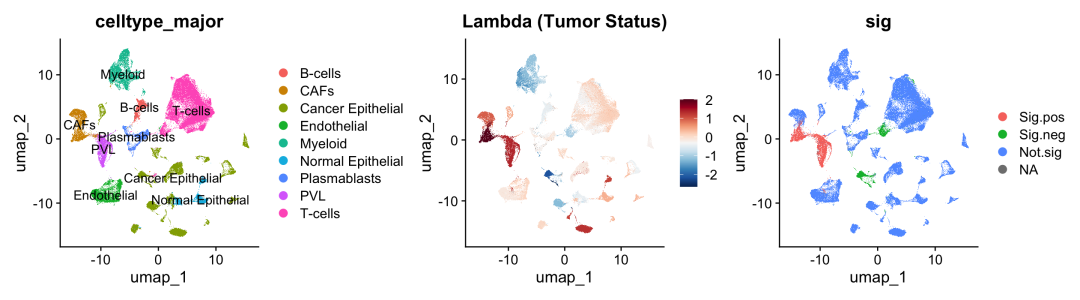 Predicted tumor status-associated cell populations
SCIPAC identifies CAFs (cancer-associated fibroblasts) and PVL (perivascular-like) cells as significantly positively associated with tumor recurrence.
2. Tumor Stage (Ordinal)
Here we use AJCC_PATHOLOGIC_TUMOR_STAGE as an ordinal phenotype.
# Tumor stage distribution
table(tcga_meta$AJCC_PATHOLOGIC_TUMOR_STAGE, useNA = "always")
#[Discrepancy]       Stage I      Stage IA      Stage IB      Stage II     Stage IIA     Stage IIB     Stage III    Stage IIIA
#            6            90            85             6             6           359           259             2           155
#   Stage IIIB    Stage IIIC      Stage IV       Stage X          <NA>
#           27            67            20            13             5

# Remove discrepant and missing entries
na.ids  <- which(is.na(tcga_meta$AJCC_PATHOLOGIC_TUMOR_STAGE))
dis.ids <- which(tcga_meta$AJCC_PATHOLOGIC_TUMOR_STAGE=="[Discrepancy]")
tcga_meta.sub <- tcga_meta[-c(na.ids, dis.ids), ]
bulk.dat.dim.redu.sub <- bulk.dat.dim.redu[rownames(bulk.dat.dim.redu) %in% tcga_meta.sub$SAMPLE_ID, ]

# Define y as an ordered factor
y <- factor(tcga_meta.sub$AJCC_PATHOLOGIC_TUMOR_STAGE)
# Verify the level ordering is correct (low to high stage)
levels(y)
#[1] "Stage I"    "Stage IA"   "Stage IB"   "Stage II"   "Stage IIA"  "Stage IIB"  "Stage III"  "Stage IIIA" "Stage IIIB"
#[10] "Stage IIIC" "Stage IV"   "Stage X"
# Confirm row name alignment
all(rownames(bulk.dat.dim.redu.sub) == rownames(y)) # TRUE
Run SCIPAC with family = "cumulative" for ordinal outcomes:
SCIPAC.res <- SCIPAC(bulk.dat = bulk.dat.dim.redu.sub, y = y,
                     family = "cumulative", ct.res = ct.res,
                     ela.net.alpha = 0.4, bt.size = 50,
                     numCores = 7, CI.alpha = 0.05, nfold = 10)
A positive Lambda indicates association with higher tumor stage; a negative Lambda indicates association with lower stage (or negative association with high stage).
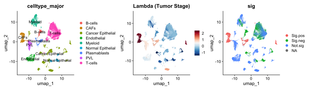 Predicted tumor stage-associated cell populations
CAF cells are significantly associated with high-grade tumors.
3. Overall Survival
For survival analysis, we use OS_STATUS (event indicator) and OS_MONTHS (follow-up time).
table(tcga_meta$OS_STATUS, useNA = "always")

# Remove samples with missing or non-positive survival times
na.ids  <- c(which(is.na(tcga_meta$OS_STATUS)), which(is.na(tcga_meta$OS_MONTHS)))
neg.ids <- which(tcga_meta$OS_MONTHS <= 0)

tcga_meta.sub <- tcga_meta[-c(na.ids, neg.ids), ]
bulk.dat.dim.redu.sub <- bulk.dat.dim.redu[rownames(bulk.dat.dim.redu) %in% tcga_meta.sub$SAMPLE_ID, ]

# Define y as a two-column data frame for Cox regression
y <- tcga_meta.sub[, c("OS_MONTHS", "OS_STATUS")]
# Encode survival status as binary (0 = living, 1 = deceased)
y$OS_STATUS <- ifelse(y$OS_STATUS == "0:LIVING", 0, 1)
# Standardize column names for SCIPAC
colnames(y) <- c("time", "status")

# Convert to numeric
y$time   <- as.numeric(y$time)
y$status <- as.numeric(y$status)
# Set row names to sample IDs
rownames(y) <- tcga_meta.sub$SAMPLE_ID
# Confirm alignment
all(rownames(bulk.dat.dim.redu.sub) == rownames(y))
Run SCIPAC with family = "cox" for survival data:
SCIPAC.res <- SCIPAC(bulk.dat = bulk.dat.dim.redu.sub, y = y,
                     family = "cox", ct.res = ct.res,
                     ela.net.alpha = 0.4, bt.size = 50,
                     numCores = 7, CI.alpha = 0.05, nfold = 10)
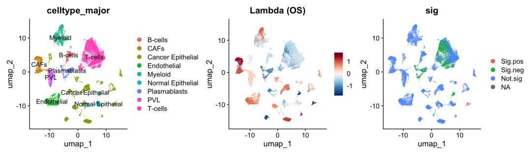 Predicted survival-associated cell populations
Interpreting Lambda in the survival setting:
- Positive Lambda (λ > 0): Associated with worse prognosis (shorter survival, higher hazard)
- Negative Lambda (λ < 0): Associated with better prognosis (longer survival, lower hazard)
⚠️ Editor's note: In Cox regression, the model estimates the log hazard ratio. Since SCIPAC uses Cox regression internally, the interpretation is:
- Positive coefficient → increased hazard → higher mortality risk → shorter survival
- Negative coefficient → decreased hazard → lower mortality risk → longer survival
In our analysis, T cells and B cells are broadly associated with better prognosis (negative Lambda), consistent with their known protective roles in anti-tumor immunity.
Other Applications
Beyond the three phenotype types demonstrated above, SCIPAC also supports general continuous outcomes — such as laboratory measurements or tumor size — by setting family = "gaussian" in the main function. In short, as long as you have relevant clinical data, SCIPAC can test associations with virtually any phenotype.
Summary
Through this complete hands-on tutorial, we have seen what SCIPAC can do:
Key Strengths Recap
- Quantitative precision — Not just "associated/not associated," but a concrete λ value for every cell
- Statistical rigor — Every result is backed by a p-value, with bootstrap-based confidence intervals
- Broad phenotype support — Binary, ordinal, survival, and continuous outcomes all handled natively
- Ease of use — The core analysis requires fewer than 20 lines of code
- Reproducibility — Built on a rigorous mathematical framework with consistent, reproducible results
What We Found
On the GSE176078 breast cancer dataset:
- Tumor recurrence: CAF and PVL cells are significantly positively associated with tumor recurrence
- Tumor stage: CAF cells are strongly associated with high-grade tumors
- Overall survival: T cells and B cells are protective factors associated with better patient survival
These findings are highly consistent with the existing literature — and crucially, we now have quantitative association strengths to underpin future mechanistic studies and clinical translation efforts.
SCIPAC vs. Scissor
| Feature | SCIPAC | Scissor |
|---|---|---|
| Output type | Quantitative λ values + p-values | Qualitative three-category classification |
| Parameter tuning | Minimal — works well out of the box | Requires iterative α tuning |
| Computational speed | Dozens of times faster | Relatively slow |
| Phenotype support | All types | Primarily binary |
| Statistical framework | Rigorous bootstrap-based inference | No formal statistical testing |
Closing Thoughts
SCIPAC represents an important step forward in single-cell data analysis — from descriptive characterization to predictive, quantitative inference. It doesn't just tell us what cells are present; it answers how strongly they relate to disease.
In the era of precision medicine, quantitative cell–phenotype association analysis will serve as a critical bridge between basic research and clinical application. As more researchers adopt SCIPAC and contribute feedback, we expect it to grow even more powerful as a tool for dissecting disease mechanisms and enabling clinical translation.
References
- GitHub repository: https://github.com/RavenGan/SCIPAC
- Original paper: Gan et al. SCIPAC: quantitative estimation of cell-phenotype associations. Genome Biology 2024
- Data sources: GSE176078 (single-cell), cBioPortal (TCGA-BRCA)
This tutorial is fully original — please credit the source if you repost. Questions and comments are welcome in the comment section!
Past highlights ⬇️:
TidyPlots in Practice: Publication-Quality Figures for RNA-seq
Stop Using Only RDS for Single-Cell Data — Give QS a Try!
The New Azimuth Might Just Be the Best Cell Annotation Tool Out There
Originally posted on WeChat Official Account: bioinfo_studyroom