Learning Single-Cell with Theis Lab: Not All Features Are Created Equal

Single-Cell Best Practices
Feature Selection
Chapter Overview — SECTION PREVIEW
1. Why feature selection is necessary and what it aims to achieve
2. Limitations of traditional methods and the new deviance-based approach
3. Hands-on: Feature selection with the scry package
This section corresponds to Chapter 8: Feature Selection in the original book
In single-cell RNA-seq data analysis, we often face a common challenge: sequencing may detect up to 30,000 genes, but many of these have zero or near-zero expression and contribute little to downstream analyses. Today, we'll learn how to use Feature Selection to identify the genes that are truly biologically meaningful, improving the efficiency of our analysis.
01
Why Do We Need Feature Selection?
After data normalization, our data has been corrected for technical noise while preserving biological variation — but a problem remains: scRNA-seq typically detects up to 30,000 genes, many of which are either not expressed or expressed at very low levels, contributing little to our understanding of cell states and types.
It's like searching for key individuals in a crowd of thousands — we need to sift through those 30,000 genes and find the "star genes" that truly reflect the biological characteristics of each cell. That's exactly what feature selection is for.
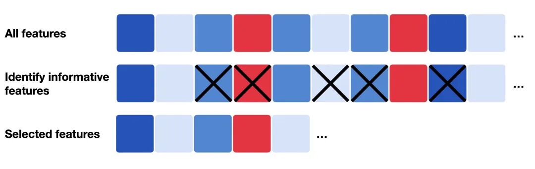
The Essence of Feature Selection
The core goal of feature selection is to identify a subset of genes that satisfies three criteria:
- • High information content: Captures the major differences between cells
- • High variability: Shows clear variation across cell types or states
- • Low noise: Not driven by random technical fluctuations
Typically, single-cell experiments focus on a specific tissue, so only a small fraction of genes exhibit biologically meaningful expression variation. Most genes are either not expressed in any cell (tissue-specific genes outside the tissue of interest) or are expressed at constant levels (housekeeping genes).
Limitations of Traditional Methods
Traditional approaches to feature selection follow two main strategies:
- Highly Variable Genes (HVGs)
- • Compute the coefficient of variation for each gene
- • Select the top 500–2,000 most variable genes
- (This is the approach used by the popular Seurat package's
FindVariableFeaturesfunction)
- Highly Expressed Genes
- • Rank genes by mean expression level
- • Select the most highly expressed genes
However, these methods have a critical flaw: remember the log1p transformation we discussed in the previous chapter? Since you can't take the logarithm of zero, a pseudocount (typically 1) is added. This seemingly harmless operation can seriously distort downstream variance calculations.
A quick note: The choice of pseudocount is arbitrary. Using 0.1, 1, or 10 yields completely different variance estimates, especially for lowly expressed genes. Studies have shown that small pseudocount values artificially inflate the variance of zero-count genes.
02
Deviance-Based Feature Selection
The Principle Behind the Deviance Approach
Germain et al. proposed an elegant solution: using deviance for feature selection. The advantages of this approach are (terminology alert ⚠️):
- Works directly on raw counts: No normalization needed, avoiding the pseudocount problem entirely
- Has a clear statistical interpretation: Deviance measures how well the data fits a null model
- Computationally simple: Can be calculated using a closed-form solution
What Is Deviance?
In simple terms, deviance quantifies whether a gene has a constant expression pattern across all cells. If a gene is expressed at roughly the same level in every cell (consistent with the null model), its deviance is low. Conversely, if a gene shows large expression differences across cells (deviating from the null model), its deviance is high.
High deviance = High information content = A gene worth paying attention to
03
Hands-On: Feature Selection with scry
First, import the required packages:
import logging
import anndata2ri
import matplotlib.pyplot as plt
import numpy as np
import rpy2.rinterface_lib.callbacks as rcb
import rpy2.robjects as ro
import scanpy as sc
import seaborn as sns

# Set up the environment
sc.settings.verbosity = 0
sc.settings.set_figure_params(
    dpi=80,
    facecolor="white",
    frameon=False,
)

# Configure the R interface
rcb.logger.setLevel(logging.ERROR)
ro.pandas2ri.activate()
anndata2ri.activate()

%load_ext rpy2.ipython
This tutorial is designed to run in a Jupyter notebook. If you prefer to run it in R (e.g., R Markdown), refer to Learning Single-Cell with Theis Lab: Format Conversion — Understanding the Underlying Logic (Part 2) for implementing the Python portions.
Load the R package:
%%R
library(scry)
Load the normalized data (i.e., the data saved in the previous chapter, Learning Single-Cell with Theis Lab: The Math Behind Normalization. If you want to jump right in, the data download link is available at the end of this article):
# Load data saved from the previous chapter
adata = sc.read(
    filename="s4d8_normalization.h5ad",
    backup_url="https://figshare.com/ndownloader/files/40015741",
)

# Pass the data to the R environment
ro.globalenv["adata"] = adata
Note: The deviance method operates on raw counts (stored in adata.X) and does not require any normalization.
Compute deviance and select features:
%%R
# Compute binomial deviance using scry
sce = devianceFeatureSelection(adata, assay="X")
Export the deviance values back to Python:
# Extract deviance values
binomial_deviance = ro.r("rowData(sce)$binomial_deviance").T
Select the top 4,000 genes by deviance:
# Sort by deviance and select the top 4000
idx = binomial_deviance.argsort()[-4000:]
mask = np.zeros(adata.var_names.shape, dtype=bool)
mask[idx] = True

# Save results to the adata object
adata.var["highly_deviant"] = mask
adata.var["binomial_deviance"] = binomial_deviance
To visualize the effect of feature selection, let's create a scatter plot of mean expression vs. dispersion for each gene:
# Compute per-gene statistics using Scanpy
sc.pp.highly_variable_genes(adata, layer="scran_normalization")

# Create the scatter plot
ax = sns.scatterplot(
    data=adata.var, x="means", y="dispersions", hue="highly_deviant", s=5
)
ax.set_xlim(None, 1.5)
ax.set_ylim(None, 3)
plt.show()
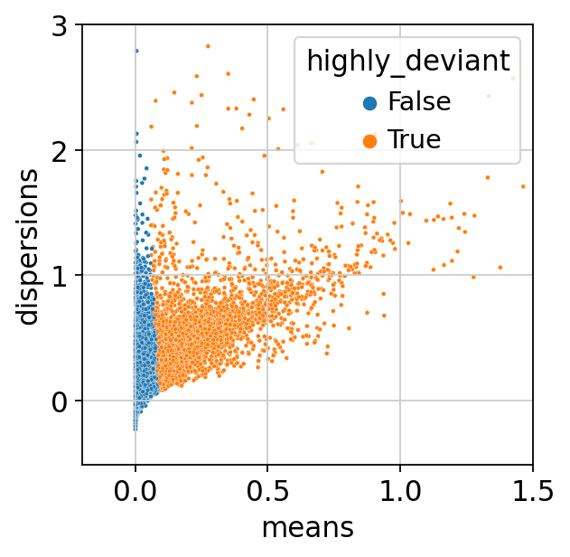 Highly deviant genes
From the plot, we can observe that genes with high mean expression tend to be selected as highly deviant genes. In real-world data, highly expressed genes are often the most biologically meaningful ones.
Finally, save the results:
adata.write("s4d8_feature_selection.h5ad")
06
Afterword
When using the deviance method, selecting 2,000–5,000 highly deviant genes is generally a good starting point. Too few genes may cause you to lose important biological signals, while too many will introduce excessive noise. Of course, the optimal number may vary depending on the tissue and experimental conditions. If you plan to perform fine-grained subpopulation analysis downstream, consider increasing the number of selected genes. You can also revisit and adjust this parameter later when evaluating clustering quality.
What do you think — does the deviance-based approach outperform traditional methods?
Originally posted on WeChat Official Account: bioinfo_studyroom