Learning Single-Cell with Theis Lab: How to Read a QC Report

Cracking single-cell analysis with Theis Lab
Series: No.03 | Published: 2025-01-17 | Estimated reading time: 13 min
**Single-Cell Best PracticesInterpreting QC Reports⭐️Chapter Overview:**1. Data QC and preprocessing2. Interpreting FastQC reports This section corresponds to Chapter 3 of the original book: Raw Data Processing 3.1
In this section, we'll explore several fundamental aspects of processing single-cell and single-nucleus RNA-seq (sc/snRNA-seq) data — a stage commonly referred to as "preprocessing." While this term is widely used, it's not entirely appropriate, since this stage involves many critical steps that make important decisions about how data is processed and represented, ultimately shaping the possibilities and limitations of downstream analysis. For clarity, we'll refer to this process as "raw data processing" throughout this section. The analysis stage we focus on here spans from lane-demultiplexed FASTQ files to the generation of a count matrix. The count matrix represents the estimated number of distinct molecules for each gene in each cell, and molecules can be further stratified by their inferred splicing status (see Figure 3.1). The resulting count matrix serves as the starting point for all downstream analyses, ranging from data normalization, integration, and filtering, to inferring cell types, developmental trajectories, and gene expression dynamics. Therefore, a reliable and accurate count matrix is essential for all subsequent analyses. Systematic estimation biases introduced during raw data processing can propagate into higher-level analyses, leading to incorrect inferences or causing signals in the data to be overlooked, weakened, or distorted. While the inputs (FASTQ files) and outputs (count matrix) of raw data processing are conceptually straightforward, several critical and challenging issues arise during implementation. More sophisticated computational methods continue to be developed to address these challenges.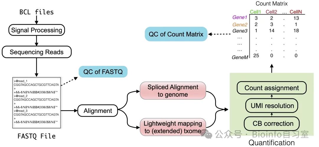
Figure 3.1: Chapter overview. "txome" stands for transcriptome.
Preliminary Note
It's worth emphasizing that our choice to start from lane-demultiplexed FASTQ files is, to some extent, an arbitrary boundary. In practice, even though FASTQ files represent a relatively early form of raw data, they are themselves the product of multiple rounds of processing and conversion from even earlier raw signals. For example, processes upstream of FASTQ generation — such as base calling and base quality assessment — affect the final quality and reliability of sequencing reads. Additionally, other issues may arise upstream of FASTQ generation, such as index hopping. However, these can be mitigated through bioinformatics approaches and the use of dual indexing. In this section, we will not delve into these upstream factors. Instead, we treat the FASTQ files converted from BCL files as the starting point of our processing pipeline and build our discussion from there.
3.1 Raw Data Quality Control
Once we have the raw FASTQ files, we can use quality control (QC) tools such as FastQC to perform a quick diagnostic assessment of read quality, sequence composition, and other metrics. When run successfully, FastQC generates a QC report for each input FASTQ file. Overall, the report summarizes quality scores, base composition, and other relevant statistics, helping us identify potential library preparation or sequencing issues. Although many modern single-cell raw data processing tools now internally evaluate certain key quality metrics (such as N content in sequences and the proportion of mappable reads), it's still worthwhile to run an independent quality check before data processing, as these assessments provide additional useful QC indicators. For readers who want to understand how FASTQ files from RNA-seq samples appear in a FastQC report, we'll walk through an example report. While this report wasn't designed specifically for single-cell data, most of its results are still informative for single-cell data — with a few caveats (discussed below). Finally, it's important to note that most metrics in these QC reports are primarily meaningful for "biological reads" (i.e., reads derived from gene transcripts). For 10x Chromium v2 and v3 datasets, these biological reads typically correspond to the read files containing "R2" in the filename. This is because technical reads consist mainly of barcode and UMI (Unique Molecular Identifier) sequences, which are not derived from the transcriptome itself and therefore should not be expected to exhibit typical biological characteristics (such as specific GC content). However, metrics like N base content remain informative even for technical reads.
Walkthrough: Interpreting a FastQC Example Report0. Summary
On the left side of the HTML report, a summary panel lists each module included in the report along with a corresponding icon for quick assessment of each section. However, since FastQC applies uniform thresholds across files generated from different sequencing platforms and biological materials, even high-quality data may receive warnings (orange exclamation marks) or failures (red crosses), while questionable data may pass (green checkmarks). Therefore, all sections/modules should be carefully evaluated before drawing conclusions about data quality.
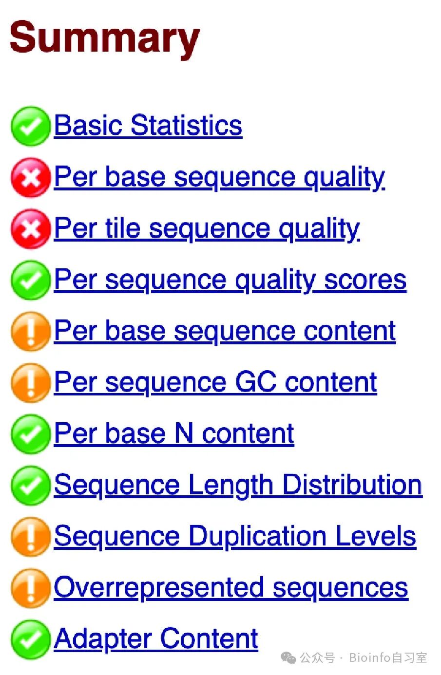
Figure 3.2: An example with somewhat poor quality.
1. Basic Statistics
The Basic Statistics module provides an overview and summary statistics for reads in the input FASTQ file, including filename, total sequence count, number of poor-quality sequences, sequence length, and overall GC content percentage across all sequences. For high-quality single-cell data, the number of poor-quality sequences should be very low, and most reads should have consistent lengths. GC content should match the overall GC content of the genome or transcriptome of the sequenced species.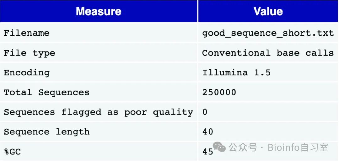
Figure 3.3: A good-quality example — note that the fifth item, "Sequences flagged as poor quality," is 0.
2. Per Base Sequence Quality
This module uses box-and-whisker plots to show the quality score distribution at each position along the reads. The x-axis represents base position along the read, and the y-axis represents quality scores. For high-quality single-cell data, the yellow boxes (representing the interquartile range of quality scores at each position) should all fall within the green zone (high quality range), and the whiskers (10th and 90th percentiles) should also remain in the green zone. Typically, quality scores decline toward the end of reads, and some bases near the read ends may fall into the orange zone (moderate quality) — this is a common signal-to-noise degradation seen in many sequencing-by-synthesis methods. However, quality boxes should never fall into the red zone (low quality). If significant low-quality bases are present, consider quality trimming the reads.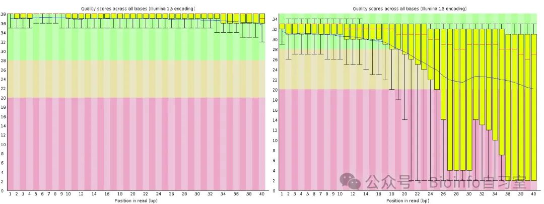
Figure 3.4: Examples of good (left) and poor (right) sequencing quality. In a good run, quality scores at the vast majority of positions should fall within the green zone.
3. Per Tile Sequence Quality
For Illumina libraries, this module plots the deviation of sequence quality from the average for each tile on the flow cell. Hotter colors indicate larger deviations. High-quality data should show a uniformly blue heatmap, indicating no significant per-tile quality deviations from the average. If only certain regions show deviations (displaying warmer colors), it suggests transient issues during sequencing, such as air bubbles passing through the flow cell or smears/debris in the imaging lane.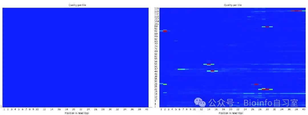
Figure 3.5: Examples of good (left) and poor (right) sequencing quality. In a good run, the entire heatmap should appear blue.
4. Per Sequence Quality Scores
This plot shows the distribution of mean quality scores across all reads/sequences in the file. The x-axis represents mean quality score, and the y-axis represents the frequency of sequences at each quality score. For high-quality data, this plot should show a single peak near the high end of the x-axis (i.e., the vast majority of sequences have high average quality). Additional peaks suggest that a subset of sequences may have quality issues.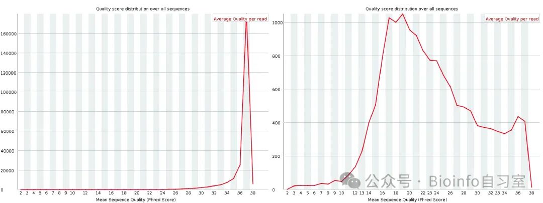
Figure 3.6: Examples of good (left) and poor (right) sequencing quality. In a good run, this plot should show only a single narrow peak on the right side of the x-axis.
5. Per Base Sequence Content
This module shows the proportion of each base (A, T, G, C) at every position across all sequences in the file. For single-cell data (and bulk RNA-seq), fluctuations at the beginning of reads are common. This is because the start of the read often corresponds to primer binding sites, which are not entirely random, leading to base composition bias. FastQC may flag this with a warning or failure, but this is very common in RNA-seq libraries and doesn't necessarily indicate a real problem.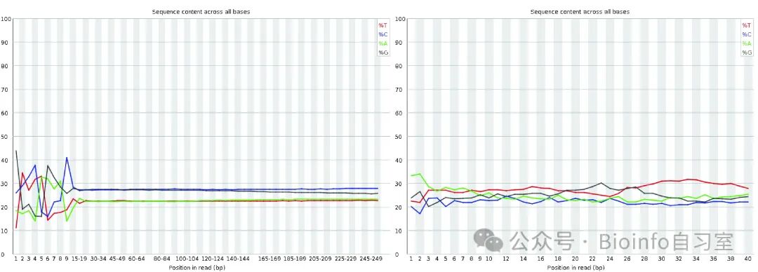
Figure 3.7: Examples of good (left) and poor (right) sequencing quality. In a good run, the base proportions should form straight, parallel lines.
6. Per Sequence GC Content
This plot shows the GC content distribution across all reads as a red curve, with the theoretical (expected) distribution shown as a blue curve. The observed peak should correspond to the overall GC content of the transcriptome. Sometimes the observed distribution is broader or narrower than the theoretical distribution — this is because the transcriptome GC content may differ from the genome, and the theoretical blue curve typically represents the genomic distribution. Even when the discrepancy triggers a warning or failure, it doesn't necessarily indicate a real problem with the transcriptome. However, if the distribution shows a complex, multimodal shape, it usually suggests library contamination. It's worth noting that in transcriptomics experiments, the GC content plot is not always easy to interpret, because in addition to the intrinsic sequence composition of the transcriptome, the (unknown) gene expression levels in the sample also influence the observed GC distribution.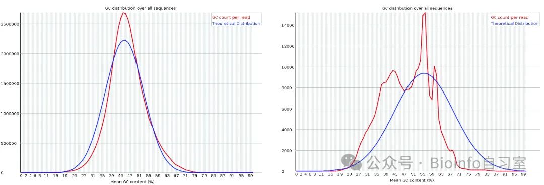
Figure 3.8: Examples of good (left) and poor (right) sequencing quality. In a good run, the red and blue curves should peak at approximately the same position (they don't need to overlap perfectly).
7. Per Base N Content
In sequencing, "N" is the placeholder assigned by the sequencer when a base cannot be confidently called. Because next-generation sequencing has inherently low error rates, high-quality libraries should not show appreciable non-zero N content at any position along the reads.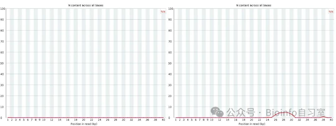
Figure 3.9: Examples of good (left) and poor (right) sequencing quality. In a good run, this plot should show a flat line near zero with no spikes.
8. Sequence Length Distribution
This module displays the distribution of sequence lengths. For most single-cell sequencing kits, all reads should be approximately the same length. If quality trimming was performed prior to the assessment, some minor variation in read length may be present. ⚠️ Tip: Bulk RNA-seq typically uses 2×150 bp paired-end sequencing, so R1 and R2 should have the same length. Single-cell sequencing is generally single-end, and the lengths of R1/R2/I1/I2 vary by chemistry version. A common configuration is R1 = 28 bp and R2 = 91 bp.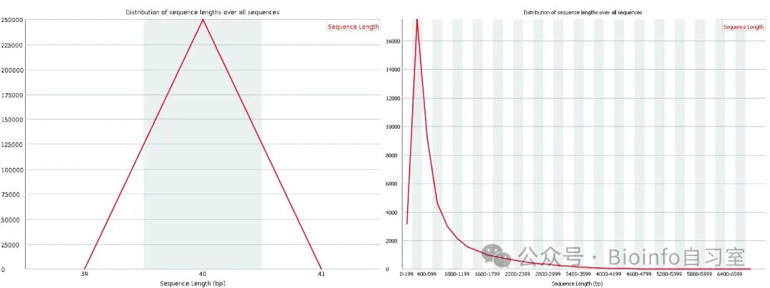
Figure 3.10: Examples of good (left) and poor (right) sequencing quality. In a good run, nearly all sequences should be the same length, appearing as a single peak with no tailing.
9. Sequence Duplication Levels
This module shows the distribution of sequence duplication levels (blue curve) and the distribution after deduplication. Because most single-cell platforms require multiple rounds of PCR amplification, and highly expressed genes produce many transcripts, and FastQC does not account for UMIs (Unique Molecular Identifiers, used to distinguish true molecular copies), it's common to see a small fraction of sequences with high duplication numbers. This may trigger a "warning" or "failure," but it doesn't necessarily indicate a data quality issue. However, the vast majority of sequences should maintain low duplication levels.
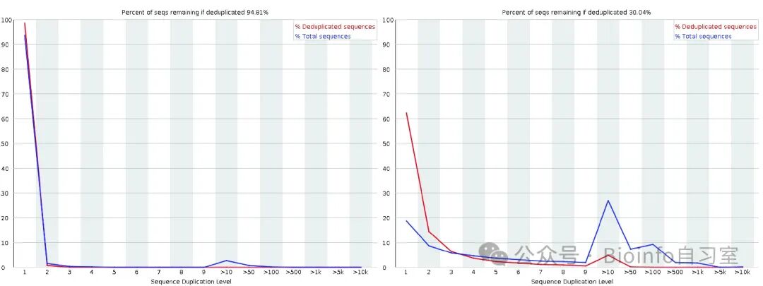 Figure 3.11: Examples of good (left) and poor (right) quality. In a good run, the vast majority of sequences should be unique, with no more than 10% showing duplication.
10. Overrepresented Sequences
This module lists read sequences that constitute more than 0.1% of total sequences. After multiple rounds of PCR amplification, highly expressed genes may produce some overrepresented sequences, but overall, most sequences should not be overrepresented. If the overrepresented sequences shown are not labeled "No Hit" (i.e., "No Hit" entries are generally not a concern), it may indicate that the library has been contaminated by the corresponding source.
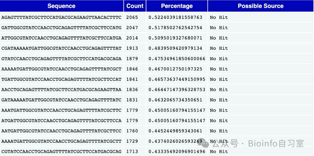 Figure 3.12: An example of overrepresented sequences. If contamination is present, the fourth column, "Possible Source," will show the suspected source.
11. Adapter Content
This module shows the cumulative proportion of each adapter sequence found in the reads, broken down by base position. Ideally, you should not see significant adapter sequence contamination in your data.
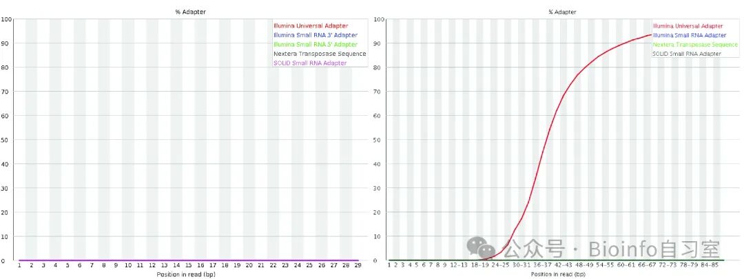 Figure 3.13: Examples of good (left) and poor (right) quality. In a good run, adapter content should be minimal (near 0).
If you have multiple FastQC reports, you can aggregate them using MultiQC. The command is straightforward (make sure MultiQC is installed beforehand):
cd fastqc  # Assuming reports are stored in a folder called "fastqc"
multiqc .
Afterword
This post corresponds to Chapter 3 of the original book. This chapter is packed with information and quite lengthy — it provides a thorough introduction to the principles and workflow of sequencing file quality control. This article primarily walked you through a detailed interpretation of the FastQC report. The remaining content is expected to be split across 4–5 additional posts. We'll update the access code and supplementary materials once everything is compiled. Thanks for following along!
Coming up next: Sequence Alignment and Mapping. Stay tuned!
Previous Posts
Learning Single-Cell with Theis Lab 02: Overview of Single-Cell SequencingUpstream Notes 1: Let's Download Data!Upstream Notes 2: Cell Ranger count Isn't That Hard
LikeShareWatchingLeave a comment
Originally posted on WeChat Official Account: bioinfo_studyroom