Learning Single-Cell Analysis with Theis Lab: The Mathematics Behind Normalization

Single-Cell Best Practices
Data Normalization
SECTION PREVIEW
1. Understand why normalization matters and what it's used for
2. Learn the theoretical foundations of normalization, including why UMI counts follow a Gamma-Poisson distribution
3. Hands-on practice: running data normalization in scanpy
This section corresponds to Chapter 7 (Normalization) of the original textbook.
⚠️ Heads up: This chapter dives into the mathematical theory behind normalization. Feel free to skip ahead to the practical section if the math isn't your thing.
In single-cell RNA sequencing (scRNA-seq) experiments, our ultimate goal is to accurately measure gene expression levels in each individual cell. However, getting from a biological sample to a final gene expression count matrix requires many complex experimental steps, each of which introduces its own technical variability:
Variability in cell capture efficiency
Different cells are captured with different efficiencies, leading to differences in the amount of starting RNA. Even cells of the same type can yield mRNA molecule counts that differ by several-fold.Variability in reverse transcription efficiency
The conversion of RNA to cDNA is influenced by many factors—including RNA length, secondary structure, and reverse transcriptase efficiency—all of which cause variation in reverse transcription efficiency across genes and cells.PCR amplification bias
During the PCR amplification step, different sequences are amplified with different efficiencies. Sequences with high GC content or unusual secondary structures may be amplified less efficiently, meaning final counts do not accurately reflect original mRNA abundance.Non-uniform sequencing depth
Even within the same sequencing run, the number of reads assigned to different cells can vary dramatically, directly affecting the sensitivity of gene detection.
The existence of these technical factors means that gene expression differences observed in the raw count matrix may not fully reflect true biological differences. Two identical cells might appear to have different expression profiles due to technical factors, while two biologically distinct cells might appear similar simply because of a large difference in sequencing depth.
Normalization addresses this problem: it removes or reduces the influence of technical variability while preserving as much true biological signal as possible. This is the foundation for all downstream analyses, including dimensionality reduction, clustering, and differential expression analysis.
In the previous chapter, we completed denoising—removing low-quality cells, ambient RNA contamination, and doublets. Now we move on to normalization. Before diving into the hands-on code, let's first explore the mathematical principles at work.
01 — Theoretical Foundations
🔬 The Gamma-Poisson Distribution
Both in theory and in practice, UMI (Unique Molecular Identifier) count data follow a Gamma-Poisson distribution (also known as the negative binomial distribution). This implies a mean-variance relationship of the form: Var = μ + μ²/θ, where μ is the mean and θ is the overdispersion parameter.
Background:
- The Gamma-Poisson distribution is a generalization of the Poisson distribution. The Poisson distribution is a discrete probability model used to describe the number of independent random events occurring within a fixed time interval, spatial region, or other unit of measurement.
- Overdispersion refers to data whose variance exceeds what the Poisson distribution predicts. When θ → ∞, the distribution reduces to a Poisson; when θ is finite, it indicates extra variability beyond Poisson noise.
- In single-cell sequencing, UMI capture, reverse transcription, and sequencing can be approximated as independent random events. Under given experimental conditions, each mRNA molecule has roughly equal probability of being detected, and since only a small fraction of total molecules are successfully captured, the data conform to the rare-event assumption of a Poisson process.
📊 Technical Variation vs. Biological Variation
In scRNA-seq data, the total observed variation can be decomposed as:
Total Variation = Biological Variation + Technical VariationBiological variation: differences in cell type, changes in cell state, true variation in gene regulatory networks
Technical variation: sequencing depth differences, capture efficiency differences, amplification bias, batch effects, etc.
The challenge of normalization is: how do we maximally remove technical variation while retaining biological variation? This requires a deep understanding of the statistical properties of the data.
🎯 Why Are Traditional Methods Insufficient?
In bulk RNA-seq, technical variation is partially averaged out because each sample contains large numbers of cells. At the single-cell level, however:
Severe zero inflation: Many genes are not expressed in any given single cell, leading to a large number of zeros in the count matrix.
Complex variance-mean relationships: Lowly expressed genes are dominated by Poisson noise, while highly expressed genes exhibit overdispersion.
Enormous intercellular differences: Total mRNA content can vary by orders of magnitude between cells.
These characteristics make traditional normalization methods (e.g., RPKM, TPM) poorly suited for single-cell data, necessitating purpose-built normalization strategies.
🎨 The Art of Normalization
The goal of normalization is to adjust for the variable sampling effects present in raw counts, scaling the observable variance into a defined range. Different normalization methods vary in complexity, but they all serve the same purpose: enabling downstream statistical analyses to work correctly.
02 — Mathematical Strategies for Normalization
💻 Setup: Importing Required Packages
import scanpy as sc
import numpy as np
import seaborn as sns
from matplotlib import pyplot as plt
import anndata2ri
import logging
from scipy.sparse import issparse
import rpy2.rinterface_lib.callbacks as rcb
import rpy2.robjects as ro

# Configure scanpy settings
sc.settings.verbosity = 0
sc.settings.set_figure_params(
    dpi=80,
    facecolor="white",
    frameon=False,
)

# Set up R interface
rcb.logger.setLevel(logging.ERROR)
ro.pandas2ri.activate()
anndata2ri.activate()
%load_ext rpy2.ipython

# Load data
adata = sc.read(
    filename="s4d8_quality_control.h5ad",
    backup_url="https://figshare.com/ndownloader/files/40014331",
)
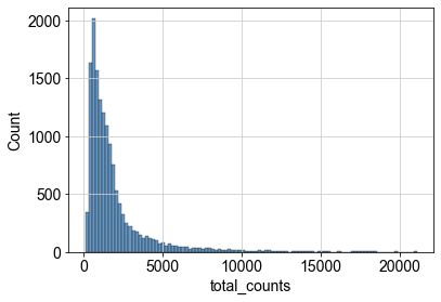
Let's first take a look at the distribution of raw counts:
p1 = sns.histplot(adata.obs["total_counts"], bins=100, kde=False)
 Source: scbp
Shifted Logarithm Normalization
The shifted logarithm sounds fancy, but it really comes down to two simple steps:
Step 1: Normalize counts
Normalized count = Raw count ÷ Size factor
Step 2: Log-transform
Final result = log(Normalized count + 1)
Background: The "+1" here is called a pseudocount, added to avoid taking the logarithm of zero (log(0) is undefined).
The size factor can be thought of as a "sequencing depth correction coefficient" for each cell, calculated as:
Size factor = Cell's total count ÷ Target total count
If a cell was sequenced deeply (high total counts), its size factor is large and its normalized counts are scaled down. Conversely, if a cell was sequenced shallowly (low total counts), its size factor is small and its normalized counts are scaled up. This brings all cells to a comparable scale.
# Perform total-count normalization (using default target sum)
scales_counts = sc.pp.normalize_total(adata, target_sum=None, inplace=False)

# Apply log1p transformation
adata.layers["log1p_norm"] = sc.pp.log1p(scales_counts["X"], copy=True)

# Visualize results
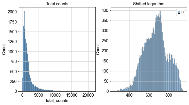
fig, axes = plt.subplots(1, 2, figsize=(10, 5))

p1 = sns.histplot(adata.obs["total_counts"], bins=100, kde=False, ax=axes[0])
axes[0].set_title("Total counts")

p2 = sns.histplot(adata.layers["log1p_norm"].sum(1), bins=100, kde=False, ax=axes[1])
axes[1].set_title("Shifted logarithm")

plt.show()
 Source: scbp
Advantages of shifted logarithm normalization:
- Fast: Computationally efficient
- Effective: Excels at revealing the underlying structure of the data, especially when combined with PCA
- Stable: Facilitates downstream dimensionality reduction and differentially expressed gene identification
scran Normalization
The scran method shares the same basic idea as the shifted logarithm, but uses a more sophisticated approach to estimating size factors.
Why the improvement?
The shifted logarithm method naively uses each cell's total count as its size factor. This has a drawback: if a cell has a few genes that are unusually highly expressed, this inflates the total count and causes other normally expressed genes to be over-corrected.
scran addresses this with a pooling strategy:
- Group: Similar cells are pooled together
- Pool-level analysis: The overall expression pattern of each pool is analyzed
- Deconvolution: Size factors for individual cells are back-calculated from the pool-level information
The benefits of this approach are:
- Reduces the influence of individual outlier genes
- Improves estimation accuracy by leveraging information from similar cells
- More robust to sparse data
from scipy.sparse import csr_matrix, issparse

# Prepare coarse clustering input for scran
adata_pp = adata.copy()
sc.pp.normalize_total(adata_pp)
sc.pp.log1p(adata_pp)
sc.pp.pca(adata_pp, n_comps=15)
sc.pp.neighbors(adata_pp)
sc.tl.leiden(adata_pp, key_added="groups")

# Prepare data for R environment
data_mat = adata_pp.X.T

# Convert to appropriate sparse matrix format
if issparse(data_mat):
    if data_mat.nnz > 2**31 - 1:
        data_mat = data_mat.tocoo()
    else:
        data_mat = data_mat.tocsc()

ro.globalenv["data_mat"] = data_mat
ro.globalenv["input_groups"] = adata_pp.obs["groups"]
%%R
library(scran)
library(BiocParallel)
# Remove temporary object
del adata_pp
%%R -o size_factors
size_factors = sizeFactors(
    computeSumFactors(
        SingleCellExperiment(
            list(counts=data_mat)),
        clusters = input_groups,
        min.mean = 0.1,
        BPPARAM = MulticoreParam()
    )
)
# Save size factors and normalize
adata.obs["size_factors"] = size_factors
scran = adata.X / adata.obs["size_factors"].values[:, None]
adata.layers["scran_normalization"] = csr_matrix(sc.pp.log1p(scran))

# Visualize results
fig, axes = plt.subplots(1, 2, figsize=(10, 5))

p1 = sns.histplot(adata.obs["total_counts"], bins=100, kde=False, ax=axes[0])
axes[0].set_title("Total counts")

p2 = sns.histplot(
    adata.layers["scran_normalization"].sum(1), bins=100, kde=False, ax=axes[1]
)
axes[1].set_title("log1p with scran-estimated size factors")

plt.show()
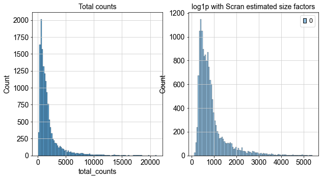
scran normalization is well suited for scenarios that involve batch effect correction or require precise size factor estimation.
Analytic Pearson Residuals
The Pearson residuals approach takes a conceptually different angle from the previous two methods. Rather than directly adjusting count values, it computes Pearson residuals. In simple terms: given a gene's average expression level and a cell's sequencing depth, we can predict how many counts that gene should have in that cell. The Pearson residual is the standardized difference between the observed count and this expected count. A positive residual means the gene is expressed higher than expected in that cell; a negative residual means lower than expected; a value near zero means the expression level matches expectations.
Compared to the previous two methods, Pearson residuals have several distinctive properties:
- No log-transformation needed: Results can be used directly, sidestepping some of the pitfalls of log transformation
- Retains full information: Negative values are meaningful and carry additional information
- Directly models technical effects: Sequencing depth is explicitly treated as a technical covariate to be regressed out
The Pearson residuals method is especially useful for finding genes that are unusually highly or lowly expressed in specific cell types, identifying rare cell types (with distinctive expression patterns), or any analysis where preserving data completeness is important.
# Compute analytic Pearson residuals
analytic_pearson = sc.experimental.pp.normalize_pearson_residuals(adata, inplace=False)
adata.layers["analytic_pearson_residuals"] = csr_matrix(analytic_pearson["X"])

# Visualize results
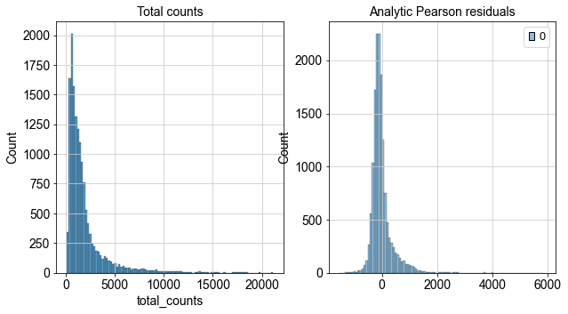
fig, axes = plt.subplots(1, 2, figsize=(10, 5))

p1 = sns.histplot(adata.obs["total_counts"], bins=100, kde=False, ax=axes[0])
axes[0].set_title("Total counts")

p2 = sns.histplot(
    adata.layers["analytic_pearson_residuals"].sum(1), bins=100, kde=False, ax=axes[1]
)
axes[1].set_title("Analytic Pearson residuals")

plt.show()
Saving Results
# Save the AnnData object with all normalization layers
adata.write("s4d8_normalization.h5ad")
Our adata object now contains three normalization layers:
log1p_norm— shifted logarithm normalizationscran_normalization— scran normalizationanalytic_pearson_residuals— analytic Pearson residuals
03 — Summary
🤔 Choosing the Right Method
According to the benchmarking study by Ahlmann-Eltze and Huber, different normalization methods perform differently depending on the task:
| Normalization Method | Best Use Case | Advantages |
|---|---|---|
| Shifted logarithm | Dimensionality reduction, differentially expressed gene identification | Fast, stable variance |
| scran normalization | Batch effect correction | Accurate size factor estimation |
| Analytic Pearson residuals | Highly variable gene selection, rare cell type identification | Preserves heterogeneity, no additional transformation needed |
📈 The Essence of Variance Stabilization
The core goal of all normalization methods is variance stabilization. In raw count data, variance is typically correlated with the mean:
- Lowly expressed genes: Dominated by Poisson noise
- Highly expressed genes: Variance grows quadratically with the mean
Normalization applies different mathematical transformations in an attempt to make the variance structure more uniform across all genes.
🎲 Understanding the Methods from a Statistical Perspective
- Shifted logarithm: Based on the delta method; achieves variance stabilization through a nonlinear transformation
- scran: A robust estimation approach based on deconvolution; the pooling strategy reduces the influence of extreme cells
- Pearson residuals: Adopts a regression framework; explicitly models and separates technical variation from biological variation
Editor's note: These three methods embody fundamentally different statistical philosophies. The shifted logarithm prioritizes simplicity and effectiveness; scran emphasizes robust parameter estimation; Pearson residuals prioritize model interpretability.
05 — Closing Thoughts
Normalization turns out to be a surprisingly deep topic in single-cell data analysis—who knew there was so much going on under the hood! That said, to state the obvious: there is no single "best" normalization method, and more complex does not always mean better. In the vast majority of cases, the simplest approach—log1p—is sufficient to make meaningful biological discoveries. Single-cell genomics is an incredibly active field, and new methods continue to emerge. But understanding the principles covered here is still tremendously valuable. We should always keep in mind that we are using idealized assumptions and simplified mathematical models to approximate gene expression in cells. Bioinformatics results should therefore be taken with a grain of salt—experimental validation remains indispensable.
Originally posted on WeChat Official Account: bioinfo_studyroom