Learning Single-Cell Analysis with Theis Lab: scanpy + muon, Your Single-Cell Swiss Army Knife

February 20, 2026 · 13 min read · Tutorials

Single-Cell Best Practices

MuData Operations Guide

SECTION PREVIEW

1. Understand the API design and functional modules of scanpy and muon

2. Master the basic single-modal data analysis workflow with scanpy

3. Learn common methods and tools for multimodal data analysis with muon

This section corresponds to Sections 4.3 Unimodal data analysis with scanpy and 4.5 Advanced: Multimodal data analysis with muon in the original book.

Scanpy

In previous chapters, we covered two key data formats: AnnData (for single-modality data) and MuData (for multi-modality data). Now it's time to learn how to actually analyze them. Within the scverse ecosystem, different packages are designed to handle different types of single-cell data:

• scanpy: primarily for RNA gene expression data analysis
• squidpy: specialized for spatial transcriptomics (gene expression with spatial coordinates)
• scirpy: focused on immune receptor data (T-cell and B-cell receptor repertoires)

While each tool has its own niche, they all draw on scanpy's core functionality — especially for data preprocessing and visualization.

scanpy is a Python toolkit built on top of AnnData for analyzing single-cell gene expression data. It provides a full suite of tools, from raw data quality control to advanced analyses, including dimensionality reduction, visualization, cell clustering, differential gene expression, and trajectory inference. Because scanpy is built on efficient Python scientific computing libraries, it can comfortably handle datasets containing millions of cells.

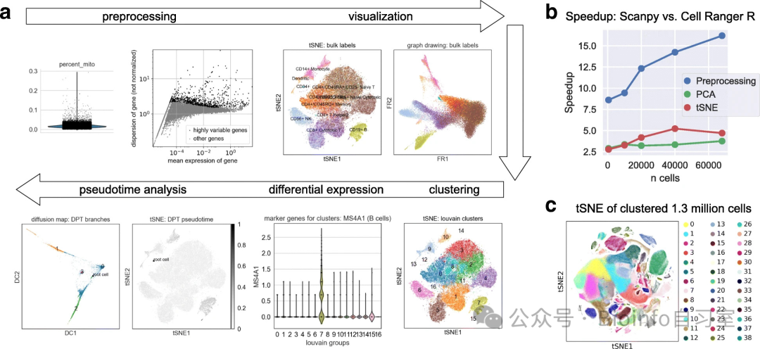scanpy overview (Source: Wolf et al., 2018)

Installing scanpy

Choose one:

pip install scanpy
# or
conda install -c conda-forge scanpy

scanpy's API Design

scanpy organizes its functions into modules — think of it as a toolbox with different drawers for different types of tools. The main modules are:

The "drawers" in the toolbox:

• sc.pp: Preprocessing module (pp = preprocessing) — data cleaning, normalization, etc.
• sc.tl: Analysis tools module (tl = tools) — dimensionality reduction, clustering, and other advanced analyses
• sc.pl: Plotting module (pl = plotting) — all visualization functions

In addition to these three main modules, data I/O functions can be called directly via sc. scanpy also provides sc.datasets, a collection of example datasets for learning and testing.

This modular design makes it easy to structure a coherent analysis pipeline: preprocess first, then apply analytical tools, and finally visualize the results.

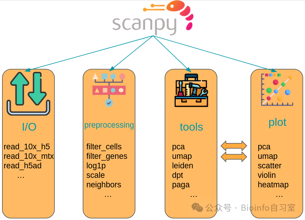scanpy API overview

⚠️ This tutorial covers only a small subset of scanpy's capabilities. Readers are encouraged to consult the official scanpy documentation for more detailed information.

A scanpy Analysis Walkthrough

Below is a brief example demonstrating the basic scanpy workflow. This is not a complete analysis — it's just meant to give you an intuitive feel for how the tool works.

We'll use an old friend: pbmc3k — 2,700 peripheral blood mononuclear cells (PBMCs) from a healthy donor. PBMCs are a mixed population of immune cells isolated from blood, widely used in immunology and drug research.

First, let's set up some basic parameters:

# Import scanpy, conventionally aliased as sc
import scanpy as sc

# Set figure parameters (resolution, background color, etc.)
sc.settings.set_figure_params(dpi=80, facecolor="white")

# Print environment info (very useful for troubleshooting)
sc.logging.print_header()

Output:

scanpy==1.9.1 anndata==0.7.8 umap==0.5.2 numpy==1.20.3 scipy==1.7.2 pandas==1.4.3 scikit-learn==1.0.1 statsmodels==0.13.1 python-igraph==0.9.10 pynndescent==0.5.5

The "header" prints the versions of all relevant packages in your environment. Version information is critical for reproducibility and debugging.

Next, let's load the 3k PBMC dataset as an AnnData object using scanpy's built-in datasets module. The data will be automatically downloaded and saved to the default data folder.

adata = sc.datasets.pbmc3k()
adata

Output:

AnnData object with n_obs × n_vars = 2700 × 32738
    var: 'gene_ids'

The returned AnnData object contains 2,700 cells and 32,738 genes. The var slot also holds gene ID annotations.

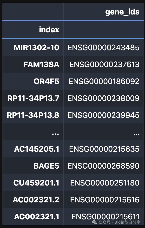adata.var output

To inspect which genes make up the highest proportion of counts per cell, we call sc.pl.highest_expr_genes, passing in the AnnData object (adata is the first argument of nearly every scanpy function) and specifying that we want the top 20 most highly expressed genes.

sc.pl.highest_expr_genes(adata, n_top=20)

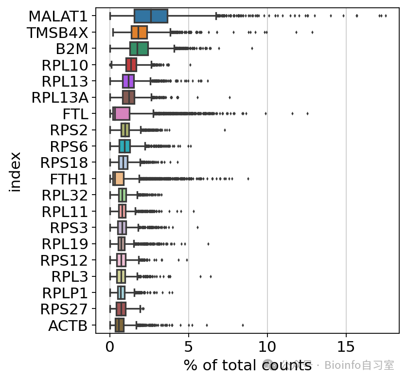Top 20 genes by expression

You'll likely notice that MALAT1 ranks among the most highly expressed genes. This is a common observation in single-cell RNA-seq, largely independent of the specific sequencing protocol used. Interestingly, MALAT1 expression tends to be negatively correlated with cell quality — higher expression may indicate a poorer cellular state.

Next, we perform basic quality control (QC) to remove likely empty droplets or low-quality cells:

# Filter cells with too few detected genes (likely empty droplets or debris)
sc.pp.filter_cells(adata, min_genes=200)

# Filter genes detected in too few cells (likely sequencing errors or non-specific signal)
sc.pp.filter_genes(adata, min_cells=3)

These two filtering steps are like selecting specimens under a microscope — discarding cells that look problematic and gene measurements that are unreliable.

⚠️ A minimum of 200 genes is not a universal gold standard; the appropriate threshold depends on the specific sample type. This will be discussed in more detail in later chapters.

Single-cell datasets typically contain tens of thousands of genes. Directly analyzing data in such high dimensions is computationally intractable, so we need dimensionality reduction — analogous to compressing a complex 3D structure into a 2D map while retaining the key features and removing noise. Principal component analysis (PCA) is the standard first step:

# Perform PCA
sc.tl.pca(adata, svd_solver="arpack")

# Visualize PCA results, colored by CST3 expression
sc.pl.pca(adata, color="CST3")

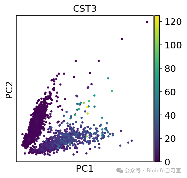PCA visualization

PCA alone isn't the most interpretable representation. To go further, we first build a neighborhood graph — identifying which cells are most similar to each other:

# Compute the neighborhood graph
sc.pp.neighbors(adata, n_neighbors=10, n_pcs=40)

With this graph in hand, we can apply UMAP, a more advanced dimensionality reduction method that produces an intuitive 2D embedding:

# Compute UMAP embedding (project high-dimensional data onto a 2D plane)
sc.tl.umap(adata)

# Visualize, coloring cells by the expression of three different genes
# Equivalent to FeaturePlot in Seurat
sc.pl.umap(adata, color=["CST3", "NKG7", "PPBP"])

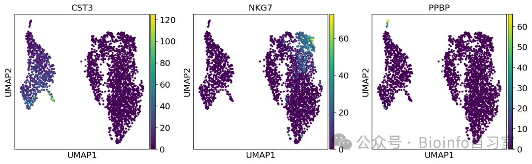UMAP visualization

In the UMAP plot, similar cells cluster together into "islands" or "communities," with color representing expression levels of different genes. These islands typically correspond to distinct cell types — T cells, B cells, monocytes, and so on.

The scanpy documentation also includes comprehensive tutorials. We recommend all readers — whether new to scanpy or brushing up — to refer to them. Video tutorials are also available on the scverse YouTube channel.

Muon

While scanpy is powerful, it was primarily designed for RNA-seq data. So how do we handle data from multiple modalities at once? That's where muon comes in.

muon extends scanpy's capabilities to specifically support the analysis of:

• ATAC-seq data (measuring chromatin accessibility — which regions of the genome are "open" and potentially active)
• CITE-seq data (simultaneously measuring cell-surface proteins and RNA)
• Multimodal data integration (combining different data types to get a more complete picture of cellular state)

muon doesn't just process each modality in isolation — it also provides specialized algorithms to extract deeper biological insights from the combination of multiple data types. It's like comparing a standard photograph, an infrared image, and an X-ray to reveal features invisible to any single view.

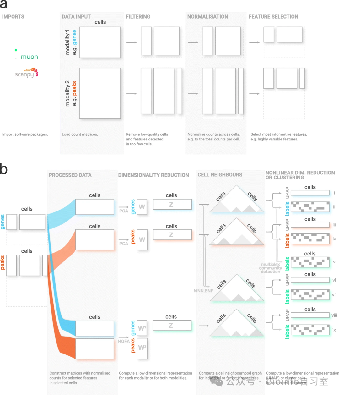muon overview (Source: Bredikhin et al., 2022)

Installing muon

muon is available via PyPI:

pip install muon

muon's Organizational Structure

muon follows a clean two-level organizational hierarchy:

By function type (mirroring scanpy):
- mu.pp: Preprocessing functions
- mu.tl: Analysis tool functions
- mu.pl: Visualization/plotting functions
By data type:
- mu.atac: Functions specialized for ATAC-seq data
- mu.prot: Functions specialized for protein (antibody-derived tag) data

This structure is like a two-dimensional library catalog: you can search by function type (fiction, science, reference) or by subject (history, biology, physics). For example, if you need preprocessing functions for ATAC data, you'll find them under mu.atac.pp.

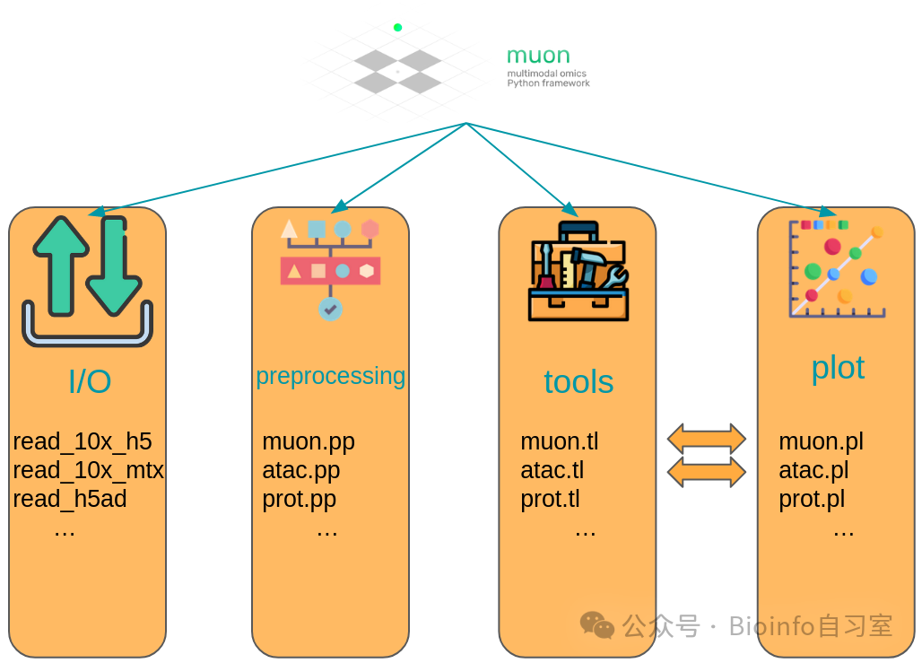muon API overview

muon in Action

Back to our old friend, PBMC. As with the previous section, this is a demonstration rather than a full analysis — the goal is simply to get you familiar with muon's basic usage. This time we're working with the 10x Genomics Multiome dataset, a cutting-edge technology that simultaneously profiles RNA expression and chromatin accessibility from the same cells.

First, let's load the data:

# Import the required libraries
import mudatasets as mds
import muon as mu

# Download and load the public PBMC multiome dataset
mdata, _ = mds.load("pbmc10k_multiome", with_info=True, full=True)

# Ensure variable names are unique to avoid downstream errors
mdata.var_names_make_unique()

This mdata object holds multiple modalities. Let's focus on the ATAC modality (chromatin accessibility data):

# Extract the ATAC modality
atac = mdata.mod["atac"]

Although ATAC and RNA data measure fundamentally different biological molecules, they share many common data quality challenges. This means we can reuse many of scanpy's general-purpose processing functions.

One important distinction: in ATAC data, instead of "genes," our features are peaks — regions of open chromatin that indicate potentially active DNA loci. Peaks in ATAC data play the same role as genes do in RNA data.

Let's perform quality control:

# Import scanpy for basic analysis
import scanpy as sc

# Compute QC metrics
sc.pp.calculate_qc_metrics(atac, percent_top=None, log1p=False, inplace=True)

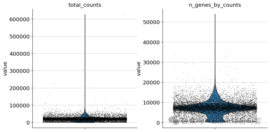
# Visualize key QC metrics with violin plots
sc.pl.violin(atac, ["total_counts", "n_genes_by_counts"], jitter=0.4, multi_panel=True)

Violin plots before filtering

After inspecting the plots, we can set filtering thresholds. First, filter out rarely detected peaks (likely background noise):

# Remove peaks detected in fewer than 10 cells
mu.pp.filter_var(atac, "n_cells_by_counts", lambda x: x >= 10)
# Check QC metrics after filtering
sc.pl.violin(atac, ["n_genes_by_counts", "total_counts"], jitter=0.4, multi_panel=True)

muon's filter_var function is more memory-efficient than scanpy's equivalent, because it modifies the data in-place rather than creating a copy.

Next, filter out low-quality cells:

# Filter cells by number of detected peaks (too few → empty droplet; too many → multiplet)
mu.pp.filter_obs(atac, "n_genes_by_counts", lambda x: (x >= 2000) & (x <= 15000))

# Filter cells by total count depth
mu.pp.filter_obs(atac, "total_counts", lambda x: (x >= 4000) & (x <= 40000))

# Re-check the distributions after filtering
sc.pl.violin(atac, ["n_genes_by_counts", "total_counts"], jitter=0.4, multi_panel=True)

⚠️ As a reminder, the QC thresholds used here are not universal — appropriate values will be discussed in detail in later chapters.

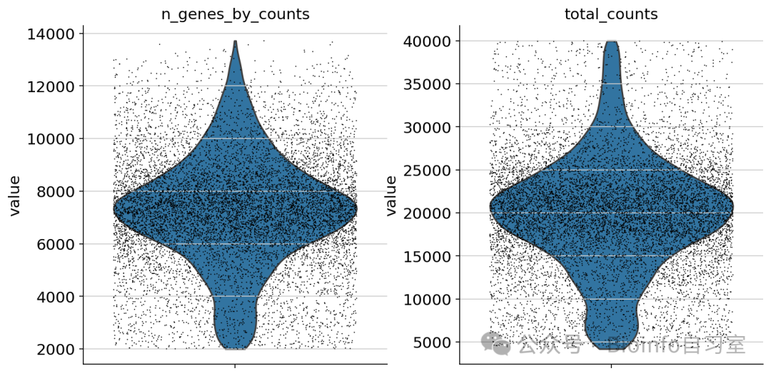After filtering

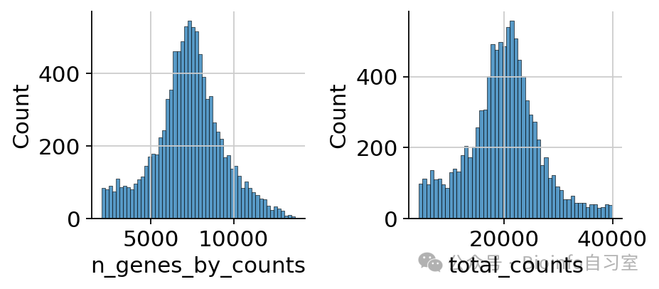
muon also offers histograms as an alternative visualization to better understand data distributions:

mu.pl.histogram(atac, ["n_genes_by_counts", "total_counts"])

Histogram

Histograms and violin plots each have their strengths: histograms clearly display the shape and modes of a distribution, while violin plots are better at showing fine distributional details and outliers.

After basic QC, we can move on to ATAC-specific analyses using muon's dedicated ATAC module:

# Import the ATAC-specific module
from muon import atac as ac

# ATAC-specific QC: compute the nucleosome signal
# (This helps assess the reliability of chromatin accessibility measurements)
atac.obs["NS"] = 1
ac.tl.nucleosome_signal(atac, n=1e6)

# Retrieve gene annotations from the RNA modality to help interpret ATAC peaks
ac.tl.get_gene_annotation_from_rna(mdata["rna"]).head(3)

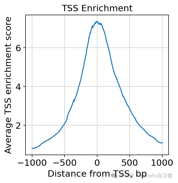
# Calculate transcription start site (TSS) enrichment
# TSS enrichment is a key quality metric for ATAC-seq data
tss = ac.tl.tss_enrichment(mdata, n_tss=1000)
ac.pl.tss_enrichment(tss)

TSS enrichment

TSS (transcription start site) enrichment analysis is critical: promoter regions are expected to be in open chromatin to allow transcription factor binding. If our ATAC data shows a clear enrichment signal at TSS regions, it indicates good data quality.

Next, we normalize the data and select informative features — steps analogous to the RNA analysis workflow:

# Save raw counts for downstream use
atac.layers["counts"] = atac.X

# Normalize each cell to the same total count depth
sc.pp.normalize_per_cell(atac, counts_per_cell_after=1e4)

# Log-transform to approximate a more normal distribution
sc.pp.log1p(atac)

# Identify highly variable features (peaks with the most dynamic signal)
sc.pp.highly_variable_genes(atac, min_mean=0.05, max_mean=1.5, min_disp=0.5)
atac.raw = atac

While PCA is often used for initial dimensionality reduction of ATAC data, Latent Semantic Indexing (LSI) is also commonly applied. LSI is available in muon's ATAC module:

# LSI dimensionality reduction
ac.tl.lsi(atac)
# From here, the workflow closely mirrors the scanpy pipeline
sc.pp.neighbors(atac, use_rep="X_lsi", n_neighbors=10, n_pcs=30)
sc.tl.leiden(atac, resolution=0.5)
sc.tl.umap(atac, spread=1.5, min_dist=0.5, random_state=20)
sc.pl.umap(atac, color=["leiden", "n_genes_by_counts"], legend_loc="on data")

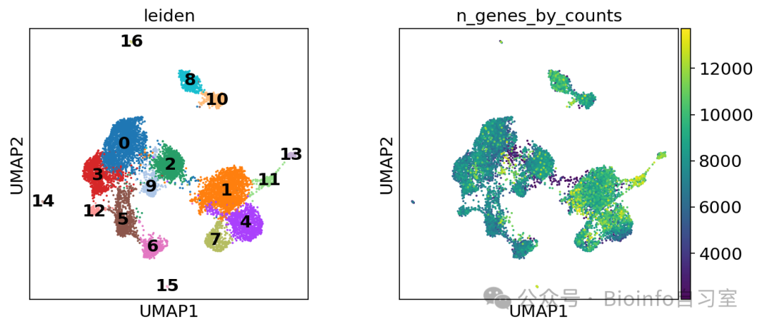UMAP UMAP

We can also use muon's ATAC module to color the UMAP by aggregated cut-site signal across peaks associated with a specific gene:

ac.pl.umap(atac, color=["KLF4"], average="peak_type")

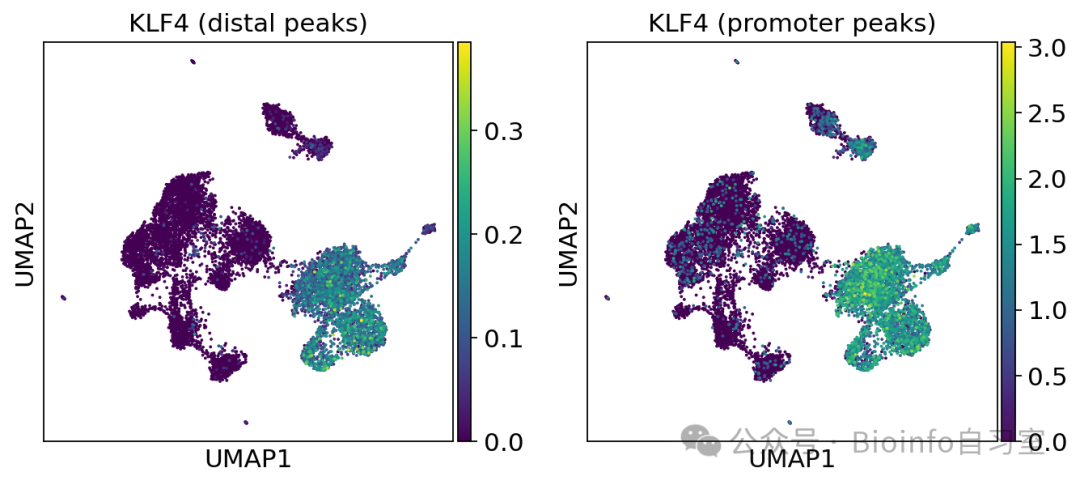KLF4 peaks

Closing Thoughts

In this installment, we introduced two important tools in the single-cell analysis landscape: scanpy and muon. They are core components of the scverse ecosystem, designed respectively for unimodal and multimodal data analysis.

Since its launch in 2018, scanpy has become one of the de facto standards for single-cell RNA-seq analysis. Its efficient implementation and rich feature set allow it to handle datasets ranging from thousands to millions of cells. In a competitive landscape, scanpy stands out in the Python ecosystem for its speed and flexibility.

As multi-omics technologies have advanced, muon emerged to fill the gap in multimodal data analysis. It inherits scanpy's design philosophy while adding dedicated support for ATAC-seq, CITE-seq, and other data types. A key strength of muon is its ability to simultaneously analyze and integrate multiple modalities — essential for capturing a comprehensive view of cellular state.

Both tools embrace a modular design, allowing users to select the most appropriate analytical methods for their needs. They integrate seamlessly with the broader Python data science ecosystem, making it easy to incorporate single-cell analyses into larger computational workflows.

The scverse ecosystem is evolving rapidly, with new tools and methods being added continuously. It's worth keeping a close eye on the official documentation and release notes to stay current with new features and best practices.

In the next tutorial, we'll explore data conversion methods between different ecosystems — specifically, how to transfer data between R and Python tools. Stay tuned!

Originally posted on WeChat Official Account: bioinfo_studyroom

Single Cell Tutorial