Learning Single-Cell Analysis with Theis Lab: Confused About Clustering vs. Dimensionality Reduction?
Single-Cell Best Practices
Clustering Analysis
SECTION PREVIEW
- Understand the biological significance and technical principles of single-cell clustering
- Grasp the core concepts of KNN graph construction and the Leiden algorithm
- Learn how to use the resolution parameter to control clustering granularity
- Hands-on practice: clustering analysis and visualization with scanpy
This section corresponds to Chapter 10 (Clustering) of the original textbook.
In previous chapters, we learned how to preprocess single-cell RNA sequencing data and visualize it after dimensionality reduction. Using methods like PCA and UMAP, we can display the distribution of cells on a two-dimensional canvas. At this stage, however, each cell is just an abstract dot — we don't yet know what type of cell it represents.
The natural next step is to identify the cellular structure within the dataset — that is, to find out which cells belong to the same type. This process is broadly referred to as cell identity annotation. To get there, we first need to group similar cells together, which is the core task of clustering analysis.
★
Dimensionality Reduction vs. Clustering
Many beginners confuse these two concepts. Simply put:
- Dimensionality reduction (e.g., PCA, UMAP) projects high-dimensional data into a low-dimensional space so that we can visualize the distribution of cells.
- Clustering groups cells based on their similarity; each group may represent a distinct cell type.
On a dimensionality-reduction plot, you may see cells gathering into clouds, but those clouds are not formally defined. Clustering algorithms explicitly delineate these groups.
The Core of Clustering: The KNN Graph
In single-cell analysis, clustering is typically performed on a k-nearest neighbor (KNN) graph. The process can be broken down into the following steps:
Compute a distance matrix: In the reduced expression space (typically the top 30–50 principal components), calculate the pairwise Euclidean distances between all cells.
Build the KNN graph:
- Each node in the graph represents a cell.
- Each cell is connected to its k most similar neighbors.
- k is typically set between 5 and 100, depending on dataset size.
Community detection: Run a community detection algorithm (such as Leiden or Louvain) on the KNN graph to identify densely connected regions.
★
Why use a KNN graph?
KNN graphs effectively capture the topological structure of the expression data. Cells that are close to each other in gene expression space will also be tightly connected in the KNN graph. This graph structure is particularly well-suited for community detection algorithms to identify cell populations.
The Leiden Algorithm: A Powerful Clustering Tool
Leiden vs. Louvain
The Leiden algorithm is an improved version of the Louvain algorithm. In multiple benchmarking studies, both algorithms significantly outperform other single-cell clustering methods. However, since the Louvain algorithm is no longer actively maintained, we recommend using Leiden.
★
Differences between Leiden and Louvain
- Louvain: An early and widely used community detection algorithm, but it has known limitations — it can produce communities with poor internal connectivity.
- Leiden: An improved algorithm introduced in 2019 that guarantees well-connected communities and produces more stable, reliable results.
- Seurat uses Louvain by default, while scanpy defaults to Leiden. However, Seurat's
FindClusters()can also use Leiden by settingalgorithm = 4.

How the Leiden Algorithm Works
Leiden creates communities by comparing the number of within-community edges to the number expected by chance across the entire graph. The algorithm proceeds as follows:
- Initial partition: Each node (cell) forms its own community.
- Node movement: Individual nodes are iteratively moved between communities to improve the partition.
- Partition refinement: The current partition is further optimized.
- Network aggregation: An aggregated network is constructed based on the refined partition.
- Iterative optimization: Steps 2–4 are repeated until no further improvement is possible.
The Resolution Parameter: Tuning Granularity
The Leiden algorithm has a key resolution parameter that controls how fine or coarse the clustering is:
- Higher resolution (e.g., 1.0, 2.0): Produces more, smaller clusters.
- Lower resolution (e.g., 0.25, 0.5): Produces fewer, larger clusters.
Choosing the right resolution is critical for downstream cell type annotation.
★
A resolution of 0.8–1.0 is generally sufficient to resolve fairly fine-grained cell populations. Alternatively, you can start with a low resolution (e.g., 0.1–0.2) and then perform sub-clustering on populations of interest to dig deeper.
Hands-On: Clustering Human Bone Marrow Cells
Let's walk through a concrete example. We'll use a single sample (site4-donor8) from the NeurIPS human bone marrow dataset.
1. Load Data and Configure Settings
import scanpy as sc

# Configure scanpy settings
sc.settings.verbosity = 0
sc.settings.set_figure_params(dpi=80, facecolor="white", frameon=False)

# Load preprocessed data
adata = sc.read("s4d8_subset_gex.h5ad")
This dataset has already been preprocessed using scran normalization, which helps us better resolve fine-grained cell states.
2. Build the KNN Graph and UMAP Embedding
# Build the KNN graph using the top 30 principal components
sc.pp.neighbors(adata, n_pcs=30)

# Compute the UMAP embedding for visualization
sc.tl.umap(adata)
★
neighborsvs.leiden
sc.pp.neighbors(): Builds the KNN graph, defining the neighborhood relationships between cells.sc.tl.leiden(): Runs the clustering algorithm on the KNN graph to assign cells to groups.The former is the prerequisite for clustering; the latter is the actual clustering step.
3. Run Leiden Clustering
We can try multiple resolution values and store each result separately:
# Default resolution (1.0)
sc.tl.leiden(adata)

# Try different resolutions and save each to a separate key
sc.tl.leiden(adata, key_added="leiden_res0_25", resolution=0.25)
sc.tl.leiden(adata, key_added="leiden_res0_5",  resolution=0.5)
sc.tl.leiden(adata, key_added="leiden_res1",    resolution=1.0)
4. Visualize Clustering Results
# Display clustering results at different resolutions on the UMAP
sc.pl.umap(
    adata,
    color=["leiden_res0_25", "leiden_res0_5", "leiden_res1"],
    legend_loc="on data",
)
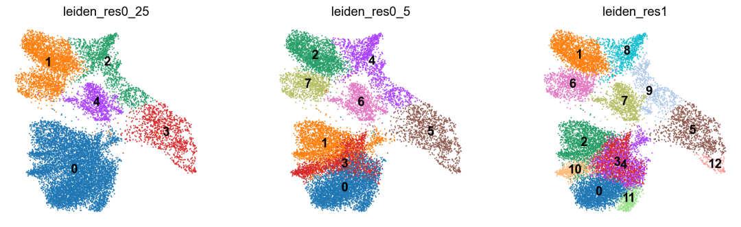
The visualization clearly demonstrates the effect of the resolution parameter:
- Resolution 0.25: Coarser clustering — fewer, broader cell populations are identified.
- Resolution 0.5: Intermediate granularity.
- Resolution 1.0: Finer clustering — more cell subpopulations are resolved.
5. An Important Caveat About Visualization
It is critical to keep in mind that distances between clusters on a UMAP plot should not be over-interpreted. Because UMAP projects high-dimensional data onto a 2D plane, distance information can be severely distorted. Do not use the spatial layout of a UMAP to infer similarity or relatedness between different cell types.
Sub-clustering: Going Deeper
The Leiden algorithm also supports sub-clustering of specific clusters. By subsetting the KNN graph to a population of interest, we can:
- Identify distinct states within a cell type
- Achieve finer cell type labels
- Uncover rare cell subpopulations
Be cautious, however: aggressive sub-clustering can lead to over-fitting, where noise is mistaken for biologically meaningful structure.
Summary
Clustering is the foundation for cell type identification: By grouping similar cells together, clustering prepares us for the downstream step of cell type annotation.
Leiden is the algorithm of choice: Graph-based community detection with the Leiden algorithm is the current standard for single-cell clustering.
Resolution matters: Choose your resolution based on your research question. Higher resolution reveals finer-grained cell subpopulations.
Interpret visualizations with caution: Distances in 2D embeddings like UMAP can be misleading — do not over-interpret the spatial relationships between clusters.
Sub-clustering adds detail: Applying clustering recursively to a population of interest can uncover finer cell states within it.
Our next step will be to learn how to biologically annotate these clusters — assigning them concrete cell type identities. This is what transforms the abstract "Cluster 3" into a meaningful label like "CD8+ cytotoxic T cell."
We've also published several annotation-focused articles on our account. Check out: Azimuth — The Most Powerful Annotation Tool We've Ever Seen
What resolution do you prefer in your own analyses? Share your experience in the comments!
The definitive single-cell tutorial series, written by the leading experts in the field, is here! Star ✨ our account to stay updated:
Previous single-cell tutorials ⬇️:
Learning Single-Cell with Theis Lab: The Mathematics Behind Normalization
Learning Single-Cell with Theis Lab: Taming High-Dimensional Data with Dimensionality Reduction
Learning Single-Cell with Theis Lab: Not All Features Are Created Equal
Originally posted on WeChat Official Account: bioinfo_studyroom