Learning Single-Cell Analysis with Theis Lab: Bridging the Batch Effect Divide (Part 1)

Single-Cell Best Practices
Data Integration (Part 1)
Chapter Overview — SECTION PREVIEW
What are batch effects, and why are they virtually unavoidable in single-cell analysis?
There are countless data integration methods — what are their similarities and differences in terms of core philosophy?
How can you smartly select highly variable genes without being misled by batch effects?
Hands-on tutorial: How to perform high-quality data integration using the star tools scVI and scANVI
This chapter corresponds to Chapter 12 (Integration), Sections 12.1–12.6 of the original book.
In the world of single-cell RNA sequencing, batch effects are a core challenge that virtually every analyst encounters. When we want to integrate data from different experimental batches, different donors, or even different laboratories to gain more comprehensive biological insights, effectively removing batch effects — letting the data "find common ground while preserving differences" — becomes the make-or-break factor for the entire analysis. This article systematically introduces the principles, methods, and practical workflow of single-cell data integration.
1. Why Do We Need Data Integration?
Simply put, batch effects refer to changes in gene expression that do not arise from biological differences but rather from variations in sample handling procedures.
Here's a classic example: Suppose two labs analyze tissue samples from the same set of donors. Lab A has optimized its tissue dissociation protocol to minimize cellular stress responses during processing, while Lab B uses a standard protocol. Even if the cells from both protocols had identical expression profiles in the original tissue, Lab B's data will likely show abnormally high expression of stress-related genes (e.g., JUN, FOS, etc.).
The sources of batch effects are varied and sometimes difficult to trace precisely. Some are purely technical — differences in sample processing workflows, reagents, sequencing depth, etc. Others are associated with biological factors, such as differences between donors, tissue regions, or sampling locations.
★
Editor's Note: Before starting your analysis, it is crucial to distinguish between technical batches and biological batches. Our goal is to remove the technical noise introduced by the former while preserving the biological signals we truly care about in the latter. For example, inter-donor variation may be a batch effect requiring correction, or it may be a key biological variable for studying disease vs. healthy states. How you define it depends on your core scientific question.
Effective data integration and batch effect removal enables us to:
- Bridge the divide between batches and identify rare cell populations that were previously obscured by noise.
- Perform cell type queries and cross-reference analyses across multiple datasets.
- Answer big-picture questions that no single dataset could address alone — for example, "Which cell types express SARS-CoV-2 entry factors across different individuals?"
How to Choose the Level of Batch Correction?
This is a critical decision that must be made before integration. Which covariate should we designate as the "batch"? The sample, the donor, or the entire dataset?
The finer the granularity of the chosen "batch," the more variation is removed — but this also greatly increases the risk of inadvertently erasing real biological signals. For example, if your samples come from different tissue regions of the same donor and you integrate at the "sample" level, the genuine biological differences between tissue regions will be "corrected" away as well. In this case, using "donor" as the batch variable may be a more sensible choice: it removes inter-individual technical variation while preserving the tissue-location differences you're interested in.
2. The Four Families of Integration Methods
The vast majority of batch correction methods follow a similar three-step logic:
- Dimensionality Reduction: Project data into a low-dimensional space to improve the signal-to-noise ratio.
- Modeling & Correction: Identify and remove batch effects in the low-dimensional space.
- Projection: Map the corrected low-dimensional data back to the high-dimensional gene expression space (optional step).
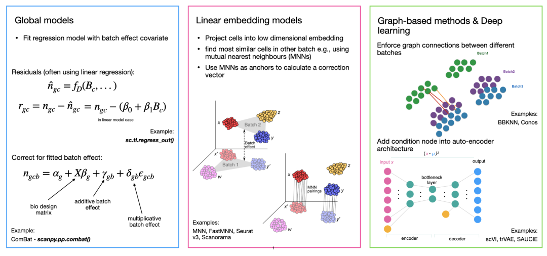 Overview of integration method categories
Based on differences in their core algorithms, we can categorize mainstream integration methods into four families:
- Global Models: Originating from microarray and bulk transcriptome analysis, these methods assume that batch effects are roughly uniform across all cells (e.g., a global additive or multiplicative shift). The classic representative is ComBat.
- Linear Embedding Models: The first generation of methods designed specifically for single-cell data. They typically first perform dimensionality reduction via SVD (Singular Value Decomposition) or similar approaches, then search for Mutual Nearest Neighbors (MNNs) between batches in the embedding space — cell pairs from different batches that are each other's closest neighbors. These MNN pairs serve as "anchors" for computing localized correction vectors. This is currently the largest family, with representatives including MNN, Seurat v3, Harmony, Scanorama, and others.
- Graph-Based Methods: These are typically the fastest. Their core idea is to force connections between cells from different batches when constructing the k-Nearest Neighbor (kNN) graph, thereby "weaving" different batches together. The most well-known representative is BBKNN.
- Deep Learning Models: The newest and most complex integration methods, which typically excel at handling large-scale, complex datasets. Most are based on autoencoder architectures that incorporate "batch" as a conditioning variable, training the model to ignore batch information when learning data structure, thereby eliminating batch effects in the low-dimensional latent space. Representative methods include scVI, scANVI, scGen, and others.
3. Hands-On Tutorial
Data Preparation and Preprocessing
In this tutorial, we'll use a publicly available 10x Multiome dataset of human bone marrow mononuclear cells. The dataset contains multiple batches; we select 3 of them, totaling 10,270 cells for downstream analysis.
import scanpy as sc
import scvi
import numpy as np
import pandas as pd

# Download data (terminal)
# wget "https://figshare.com/ndownloader/files/45452260" -O openproblems_bmmc_multiome_genes_filtered.h5ad

# Read data
adata = sc.read_h5ad("openproblems_bmmc_multiome_genes_filtered.h5ad")

label_key = "cell_type"  # Cell type labels
batch_key = "batch"       # Batch information

# Select the three batches we'll use
keep_batches = ["s1d3", "s2d1", "s3d7"]
adata = adata[adata.obs[batch_key].isin(keep_batches)].copy()

# This tutorial focuses on gene expression (GEX) only; filter out ATAC and other modalities
adata = adata[:, adata.var["feature_types"] == "GEX"].copy()

# Remove genes not expressed in any cell
sc.pp.filter_genes(adata, min_cells=1)

# Place the raw count matrix back into adata.X — the recommended input for many integration methods (especially scVI)
adata.X = adata.layers["counts"].copy()

# Re-normalize and log-transform for visualization and methods that don't use raw counts
sc.pp.normalize_total(adata)
sc.pp.log1p(adata)
Inspecting the Unintegrated Data
Before diving into integration, we must first visually assess how severe the batch effects are in the raw data.
# Standard preprocessing pipeline
sc.pp.highly_variable_genes(adata)
sc.tl.pca(adata)
sc.pp.neighbors(adata)
sc.tl.umap(adata)

# Color UMAP by both cell type and batch
sc.pl.umap(
    adata,
    color=[label_key, batch_key],
    wspace=0.5  # Adjust subplot spacing
)
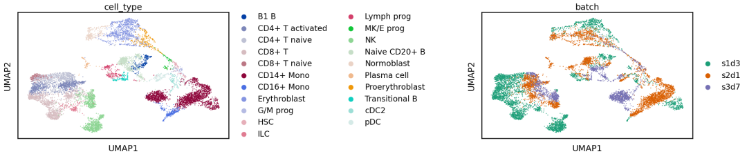 Unintegrated data showing clear batch effects
The UMAP clearly shows that although some cell types (e.g., HSC) partially overlap across batches, most cells are visibly separated by their source batch (batch) rather than clustering by their biological identity (cell_type). This is the classic signal that batch correction is needed.
Batch-Aware Feature Selection (Batch-Aware HVG Selection)
Before dimensionality reduction and integration, we need to select the most informative genes — highly variable genes (HVGs). However, in data containing multiple batches, traditional HVG selection methods can make a critical mistake: they may select genes that are "spuriously" highly variable due to batch effects (e.g., stress-response genes activated only in a specific batch).
A more robust approach is batch-aware HVG selection:
- Compute HVGs independently within each batch.
- Select genes that are identified as highly variable across as many batches as possible as the final gene set.
Scanpy's highly_variable_genes function makes this straightforward by setting the batch_key parameter.
sc.pp.highly_variable_genes(
    adata,
    n_top_genes=2000,
    flavor="cell_ranger",   # Classic HVG calculation method
    batch_key=batch_key     # Key parameter!
)

# Create an AnnData object containing only HVGs for downstream integration
adata_hvg = adata[:, adata.var["highly_variable"]].copy()
★
Editor's Note: How many HVGs should you select? The scvi-tools developers recommend between 1,000 and 10,000 genes. Too few, and you risk losing key marker genes that define rare cell populations; too many, and you significantly increase the computational burden. A safer strategy is to err on the side of more (e.g., 3,000–5,000) rather than fewer.
Variational Autoencoder (VAE)-Based Integration: scVI
scVI (single-cell Variational Inference) is one of the most popular deep learning-based integration methods today. It is built on a Conditional Variational Autoencoder (CVAE). The core idea is to feed "batch information" into the model as a known condition when modeling the raw expression counts of genes. This way, during dimensionality reduction (compressing from high-dimensional gene space to low-dimensional latent space), the model learns to "ignore" batch information, so the resulting low-dimensional embedding (latent representation) is no longer affected by batch effects.
1. Prepare data for scVI
scVI has a standard data setup workflow handled through the setup_anndata function. This step tells the model where to find the required data (e.g., raw counts) and which batch variable to correct for.
adata_scvi = adata_hvg.copy()

# Set up the scVI model
scvi.model.SCVI.setup_anndata(
    adata_scvi,
    layer="counts",       # Explicitly specify raw count matrix
    batch_key=batch_key
)
2. Build and train the model
# Create scVI model instance
model_scvi = scvi.model.SCVI(adata_scvi)

# Train the model
# The tutorial provides a method to dynamically set training epochs to adapt to datasets of varying sizes
# Basic idea: total training iterations ≈ 20000 × 400, divided by the number of cells to get epochs
max_epochs = np.min([round((20000 / adata.n_obs) * 400), 400])
model_scvi.train(max_epochs=max_epochs)

# After training, extract the integrated low-dimensional embedding from the model
adata_scvi.obsm["X_scVI"] = model_scvi.get_latent_representation()
3. Visualize the integration results
Now we recompute the neighbor graph and UMAP based on the integrated X_scVI embedding.
# Compute the kNN graph using the integrated embedding (X_scVI)
sc.pp.neighbors(adata_scvi, use_rep="X_scVI")
sc.tl.umap(adata_scvi)

# Visualize again
sc.pl.umap(
    adata_scvi,
    color=[label_key, batch_key],
    wspace=0.5,
    title=["Cell Type (scVI integrated)", "Batch (scVI integrated)"]
)
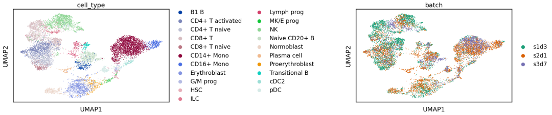 Data after scVI integration
You can see that after scVI integration, batch effects on the UMAP have essentially disappeared. Cells from different batches are well mixed, and cell types that were previously separated by batch (e.g., CD4 T cells) are now successfully clustered together.
Further Refinement with Cell Labels: scANVI
If we already have type labels for some (or even all) cells, we can use scANVI (single-cell ANnotation using Variational Inference) to achieve even higher-quality integration. scANVI extends the scVI model by additionally leveraging cell label information as a supervisory signal, enabling it to better preserve the biological differences that define cell types while removing batch effects.
Training the scANVI Model
scANVI training is typically a fine-tuning process — continuing training from a pre-trained scVI model — which greatly reduces computation time.
# Create scANVI model based on the trained scVI model
model_scanvi = scvi.model.SCANVI.from_scvi_model(
    model_scvi,
    labels_key=label_key,
    unlabeled_category="unlabelled"  # Specify a label for unannotated cells, if any
)

# Train scANVI model (usually requires fewer epochs)
max_epochs_scanvi = int(np.min([10, np.max([2, round(max_epochs / 3.0)])]))
model_scanvi.train(max_epochs=max_epochs_scanvi)

# Extract scANVI-integrated embeddings
adata_scanvi = adata_scvi.copy()  # For easy comparison
adata_scanvi.obsm["X_scANVI"] = model_scanvi.get_latent_representation()

# Visualize
sc.pp.neighbors(adata_scanvi, use_rep="X_scANVI")
sc.tl.umap(adata_scanvi)
sc.pl.umap(adata_scanvi, color=[label_key, batch_key], wspace=1)
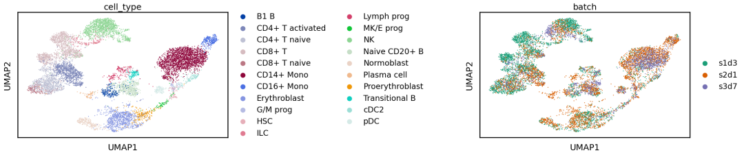 Data after scANVI integration
Extensive benchmarking has shown that scANVI generally preserves biological signals better than scVI, though sometimes at the cost of slightly weaker batch correction. Notably, scANVI also supports semi-supervised mode, where only a subset of cells carry reliable labels — a very practical feature for real-world projects.
Closing Thoughts
In this article (Part 1), we explored the sources of batch effects, the necessity of data integration, and provided a detailed introduction to two powerful deep learning-based integration tools — scVI and scANVI. These methods excel at handling complex, large-scale datasets and offer good scalability, though they do require substantial computational resources (especially a GPU).
In the next article (Part 2), we will introduce two other mainstream approaches — the graph-based method BBKNN and the linear embedding-based method MNN — and discuss how to quantitatively evaluate integration quality. Stay tuned!
What's your experience with batch effect removal? Which tools work best, and which tend to overfit? Feel free to share your thoughts in the comments! To access the original English text and complete code for this chapter, reply scbp12 in the backend.
All bioinformatics enthusiasts are welcome to join the Bioinfo Study Room community:
Originally posted on WeChat Official Account: bioinfo_studyroom