Learning Single-Cell Analysis with Theis Lab: An Introduction to AnnData

February 20, 2026 · 13 min read · Tutorials

Best Practices in Single-Cell Analysis

An Introduction to AnnData

SECTION PREVIEW

Understand the major single-cell analysis ecosystems and their differences
Install AnnData and learn the basic structure for storing unimodal data
Master the fundamental operations of AnnData

This section corresponds to Sections 4.1 (Single-cell analysis frameworks and consortia) and 4.2 (Storing unimodal data with AnnData) of the original book.

01 — Downstream Single-Cell Analysis

"Downstream" single-cell analysis generally refers to the exploratory analysis that begins once a count matrix has been obtained. Because of the unique properties of single-cell data — sparsity (the vast majority of matrix entries are zeros), large scale (ranging from thousands to millions of cells), and low signal-to-noise ratio (due to empty droplets, multiplets, ambient RNA, and dropout events) — off-the-shelf tools are rarely sufficient. Early researchers typically wrote their own analysis scripts from scratch, but today there are dedicated frameworks designed specifically for single-cell data. The three most popular choices are the R-based Bioconductor and Seurat ecosystems, and the Python-based scverse. These frameworks differ not only in programming language, but also in their underlying data structures and the suite of analysis tools they provide.

Bioconductor is a project dedicated to developing, supporting, and sharing free, open-source software for rigorous and reproducible analysis of biological data, including single-cell data. Its greatest strengths are a consistent developer and user experience and well-written vignettes that help users get up to speed quickly.
Seurat is a widely acclaimed R package designed specifically for single-cell data analysis. It provides a comprehensive toolkit spanning data preprocessing, multimodal analysis, and spatial transcriptomics. Seurat excels through its detailed vignettes and large user community. However, when dealing with very large datasets (e.g., more than 500,000 cells), both R-based options (Bioconductor and Seurat) may face scalability challenges — a limitation that motivated the Python community to develop the scverse ecosystem.
scverse is an organization and ecosystem focused on foundational tools for the life sciences, with an initial emphasis on single-cell data analysis. Its strengths lie in excellent scalability, flexibility, and strong interoperability with existing Python data science and machine learning libraries.

While all three ecosystems cover the core analytical functions, active efforts are underway to enable "seamless interoperability" between frameworks, giving users the flexibility to choose the right tool for the problem at hand. This book will select the most appropriate tool for each task, drawing on multiple frameworks, but all analyses will be built on the scverse ecosystem to maintain a consistent data structure. We will focus on the underlying concepts rather than implementation details; for the latter, readers are encouraged to consult the official documentation and tutorials.

02 — Storing Unimodal Data with AnnData

As mentioned earlier, after read alignment and gene annotation, genomic data are typically summarized into a feature matrix. For single-cell RNA sequencing (scRNA-seq) data, this matrix has shape n_obs × n_vars, where observations correspond to cell barcodes and variables correspond to annotated genes — in plain terms, it is a cells × genes matrix. During analysis, we add computed measurements (e.g., QC metrics or latent-space embeddings) and prior knowledge (e.g., sample of origin or alternative gene identifiers) to both the observations and variables.

In the scverse ecosystem, AnnData is the core data structure that links the data matrix to these annotations. To maximize efficiency, AnnData supports sparse matrices and partial I/O (reading only parts of the data on demand), enabling fast processing of large-scale datasets.

AnnData is functionally analogous to data structures in the R ecosystem — such as Bioconductor's SummarizedExperiment or the Seurat object — but note that R packages typically store the transposed feature matrix (genes × cells).

The Core Structure of AnnData

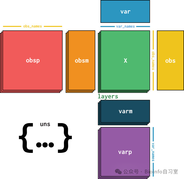
AnnData data structure diagram

At the core of an AnnData object is a sparse or dense matrix — the count matrix in the case of scRNA-seq — stored as X. Its dimensions are obs_names × var_names, where obs (observations) corresponds to cell barcodes and var (variables) corresponds to gene identifiers. The matrix X is flanked by two Pandas DataFrames: obs stores per-cell annotation, and var stores per-gene annotation.

AnnData can also store a wealth of additional information:

obsm / varm: multi-dimensional arrays associated with observations or variables (e.g., UMAP embeddings)
obsp / varp: graph structures capturing relationships between cells or between genes
uns: unstructured metadata that does not fit elsewhere (e.g., experimental design, color palettes)
layers: alternative representations of the core matrix X — for example, raw (un-normalized) counts can be stored in a layer called counts, while the default matrix holds normalized values

AnnData is primarily designed for unimodal data (e.g., scRNA-seq alone). However, its extension MuData (introduced later) can efficiently store and access multimodal data.

03 — Core AnnData Operations

Installation

Either of the following commands will install AnnData along with its dependencies:

# Using conda
conda install -c conda-forge anndata
# Using pip
pip install anndata

Initialization

Suppose we want to store gene expression count data (e.g., from scRNA-seq). Here is how to create an AnnData object step by step.

First, import the required libraries:

import anndata as ad
import numpy as np
import pandas as pd
from scipy.sparse import csr_matrix

Next, generate some random data to simulate a gene expression count matrix and use it to initialize an AnnData object called adata:

# Create a sparse matrix simulating gene expression counts
counts = csr_matrix(
    np.random.default_rng().poisson(1, size=(100, 2000)), dtype=np.float32
)
# Initialize the AnnData object
adata = ad.AnnData(counts)
adata

AnnData object with n_obs × n_vars = 100 × 2000

This tells us the data has 100 observations (cells) and 2,000 variables (genes). The underlying matrix is accessible via adata.X:

adata.X

<100x2000 sparse matrix of type '<class 'numpy.float32'>'
    with 126413 stored elements in Compressed Sparse Row format>

To make the object more interpretable, we can assign meaningful names to cells and genes, stored in .obs_names and .var_names:

# Name the cells and genes
adata.obs_names = [f"Cell_{i}" for i in range(adata.n_obs)]
adata.var_names = [f"Gene_{i}" for i in range(adata.n_vars)]

print(adata.obs_names[:10])  # Print the first 10 cell names

Index(['Cell_0', 'Cell_1', 'Cell_2', 'Cell_3', 'Cell_4', 'Cell_5', 'Cell_6',
       'Cell_7', 'Cell_8', 'Cell_9'],
      dtype='object')

Annotations

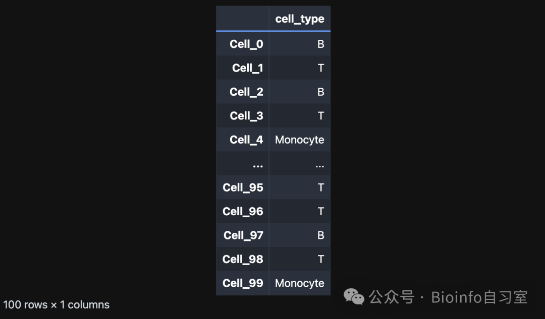
In single-cell data analysis, cells and genes typically carry additional annotation — such as cell type or gene function. This information can be added to the AnnData object via the .obs and .var attributes. For example, we can randomly generate cell-type labels and store them in .obs:

# Randomly assign cell-type labels
cell_types = np.random.default_rng().choice(["B", "T", "Monocyte"], size=adata.n_obs)
adata.obs["cell_type"] = pd.Categorical(cell_types)  # Use Categorical for efficiency
# AnnData updates automatically
adata

AnnData object with n_obs × n_vars = 100 × 2000
    obs: 'cell_type'

You can also inspect .obs directly:

adata.obs

Subsetting

We can filter the data based on annotation. For example, to extract all B cells:

bdata = adata[adata.obs.cell_type == "B"]
bdata

View of AnnData object with n_obs × n_vars = 26 × 2000
    obs: 'cell_type'

Multi-Dimensional Annotations

Some annotations are inherently multi-dimensional, such as UMAP embeddings or gene-level factor loadings. These can be stored in .obsm and .varm, respectively.

For example, we can generate random UMAP coordinates and store them in .obsm:

# Store UMAP embedding
adata.obsm["X_umap"] = np.random.default_rng().normal(0, 1, size=(adata.n_obs, 2))
# Store gene-level metadata
adata.varm["gene_stuff"] = np.random.default_rng().normal(0, 1, size=(adata.n_vars, 5))
# Inspect the obsm slot
adata.obsm

AxisArrays with keys: X_umap

# View the updated AnnData
adata

AnnData object with n_obs × n_vars = 100 × 2000
    obs: 'cell_type'
    obsm: 'X_umap'
    varm: 'gene_stuff'

Two things to keep in mind about .obsm and .varm: (1) These slots accept array-like metadata — Pandas DataFrames, scipy sparse matrices, or NumPy dense arrays are all valid. (2) When using scanpy, data stored in these slots cannot be directly passed to plotting functions. If you need to plot the data, store it in .obs instead.

Unstructured Metadata

For information that does not fit neatly into other slots, use the .uns attribute. There are no format restrictions — you can store anything here, such as experimental design notes, reagent versions, or color palettes. That said, if data can be stored in a typed slot, prefer that over .uns. Let's try it out:

adata.uns["random"] = [1, 2, 3]
adata.uns

# Stored as a dictionary
OverloadedDict, wrapping:
    OrderedDict([('random', [1, 2, 3])])
With overloaded keys:
    ['neighbors'].

Data Layers

If you have multiple representations of the same data (e.g., raw counts and normalized counts), you can store them in separate layers. For example, we can log-transform the raw matrix and save the result as a new layer:

adata.layers["log_transformed"] = np.log1p(adata.X)
adata

AnnData object with n_obs × n_vars = 100 × 2000
    obs: 'cell_type'
    uns: 'random'
    obsm: 'X_umap'
    varm: 'gene_stuff'
    layers: 'log_transformed'

Writing to a new layer does not modify the original data. Let's verify:

# Compare X and the log_transformed layer
(adata.X != adata.layers["log_transformed"]).nnz == 0
# False

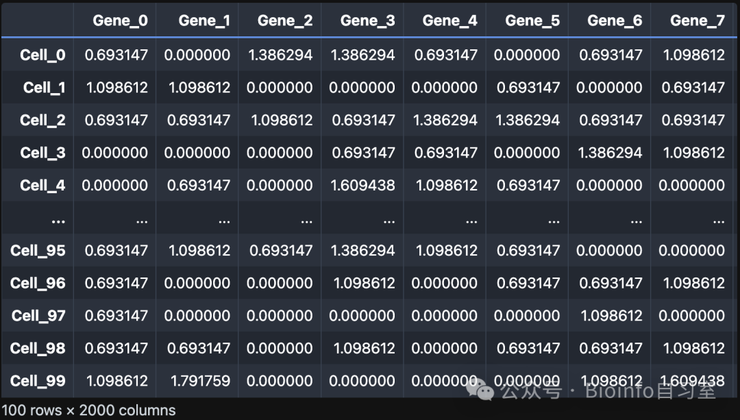
You can also export a layer as a Pandas DataFrame:

adata.to_df(layer="log_transformed")

Reading and Writing

AnnData objects are typically saved as .h5ad files — a variant of the HDF5 format. The key advantages of this format are its hierarchical data structure, built-in compression, and efficient on-disk representation that mirrors the in-memory layout, enabling fast read/write operations. Let's save our AnnData object:

# Write to an h5ad file
adata.write("my_results.h5ad", compression="gzip")
# Inspect the on-disk structure
!h5ls 'my_results.h5ad'

X                        Group
layers                   Group
obs                      Group
obsm                     Group
uns                      Group
var                      Group
varm                     Group

...and then read it back:

adata_new = ad.read_h5ad("my_results.h5ad")
adata_new

AnnData object with n_obs × n_vars = 100 × 2000
    obs: 'cell_type'
    uns: 'random'
    obsm: 'X_umap'
    varm: 'gene_stuff'
    layers: 'log_transformed'

Views vs. Copies

To better understand AnnData's data access model, consider a typical metadata scenario: suppose observations come from multiple instruments, measurements were collected over 10 years, and samples were drawn from different subjects at different sites. We would normally receive this information in some tabular format and store it in a Pandas DataFrame:

obs_meta = pd.DataFrame(
    {
        "time_yr": np.random.default_rng().choice([0, 2, 4, 8], adata.n_obs),
        "subject_id": np.random.default_rng().choice(
            ["subject 1", "subject 2", "subject 4", "subject 8"], adata.n_obs
        ),
        "instrument_type": np.random.default_rng().choice(
            ["type a", "type b"], adata.n_obs
        ),
        "site": np.random.default_rng().choice(["site x", "site y"], adata.n_obs),
    },
    index=adata.obs.index,  # Using the same cell IDs as before
)

We then combine this metadata with the expression matrix to create a complete data container:

adata = ad.AnnData(adata.X, obs=obs_meta, var=adata.var)
adata

AnnData object with n_obs × n_vars = 100 × 2000
    obs: 'time_yr', 'subject_id', 'instrument_type', 'site'

AnnData objects behave similarly to NumPy arrays: they can store actual data, or they can reference another AnnData object (called a "view"). When you slice an AnnData object, the result is a view rather than a copy of the data. This is one of the key differences from R, which creates a new object when you perform the same operation. Views offer two advantages:

No new memory is allocated.

Modifications propagate directly to the underlying AnnData object.

If you need a fully independent AnnData object, you can materialize the view by calling .copy(). In practice this is usually unnecessary, because modifying an element of a view automatically triggers an internal .copy() call.

# Get a view of the first 5 cells and two specific genes
adata_view = adata[:5, ["Gene_1", "Gene_3"]]
adata_view

View of AnnData object with n_obs × n_vars = 5 × 2
    obs: 'time_yr', 'subject_id', 'instrument_type', 'site'

Inspecting the original adata confirms that its dimensions are unchanged:

adata

AnnData object with n_obs × n_vars = 100 × 2000
    obs: 'time_yr', 'subject_id', 'instrument_type', 'site'

To create a fully independent (non-view) AnnData object, call .copy() explicitly:

adata_subset = adata[:5, ["Gene_1", "Gene_3"]].copy()

You can also modify data through a view. For example, setting the first 3 values of Gene_1 to zero:

print(adata[:3, "Gene_1"].X.toarray().tolist())
adata[:3, "Gene_1"].X = [0, 0, 0]
print(adata[:3, "Gene_1"].X.toarray().tolist())

[[0.0], [2.0], [1.0]]
[[0.0], [0.0], [0.0]]

However, when you try to modify (or read from) a part of a view, the contents are automatically copied and the result becomes an independent AnnData object — no longer a view:

adata_subset = adata[:3, ["Gene_1", "Gene_2"]]
adata_subset

View of AnnData object with n_obs × n_vars = 3 × 2
    obs: 'time_yr', 'subject_id', 'instrument_type', 'site'

# Attempt to modify the view
adata_subset.obs["foo"] = range(3)
# adata_subset is now an independent AnnData object
adata_subset

Trying to set attribute `.obs` of view, copying.
AnnData object with n_obs × n_vars = 3 × 2
    obs: 'time_yr', 'subject_id', 'instrument_type', 'site', 'foo'

Flexible Subsetting with Pandas

We can also leverage Pandas to subset the data using sequences or boolean indices:

adata[adata.obs.time_yr.isin([2, 4])].obs.head()

        time_yr subject_id instrument_type    site
Cell_0        4  subject 8          type b  site x
Cell_2        2  subject 2          type b  site y
Cell_3        4  subject 8          type a  site y
Cell_5        2  subject 2          type a  site y
Cell_10       2  subject 8          type b  site x

Partial Loading of Large Files

If a single .h5ad file is very large, you can use backed mode or read_elem to load only part of the data into memory:

adata = ad.read("my_results.h5ad", backed="r")
adata.isbacked  # Check whether backed mode is active

True

In this mode, the AnnData object maintains a live connection to the file on disk:

adata.filename

PosixPath('my_results.h5ad')

Since we opened the file in read-only mode, no modifications can be accidentally written to disk. However, once you are done with the file, be sure to close the connection:

adata.file.close()

04 — Closing Thoughts

In this installment we took a detailed look at the structure and core operations of the Python AnnData object — arguably the most important foundation for everything that follows in single-cell analysis. Build this foundation well and the rest becomes much easier.

The author works primarily in R, but writing up this tutorial made the view/copy distinction genuinely fascinating: it is precisely this mechanism that allows Python to handle large-scale data so efficiently. Interestingly, Seurat is also adopting a similar approach — the BPCells backend introduced in Seurat v5.0 works on the same principle, maintaining a direct link to on-disk files and reading/writing without ever fully loading the data into RAM, which dramatically reduces memory usage and speeds up computation. We plan to cover this in a future tutorial!

Next time, we will reorganize the chapter order slightly: first introducing the multimodal data structure MuData and its operations, then walking through a basic scanpy and muon workflow with a hands-on example. The "Introduction" chapter of the original book also covers cross-ecosystem conversion methods — something many readers have asked about.

The "Introduction" section of the book provides a concise overview of single-cell technology and the full upstream/downstream pipeline. More in-depth discussions follow on the details of each downstream analysis step (e.g., choosing QC thresholds and tuning parameters) as well as advanced topics such as trajectory inference, pathway enrichment analysis, and gene regulatory networks. Don't miss it if you are working toward a systematic mastery of single-cell analysis!

Originally posted on WeChat Official Account: bioinfo_studyroom

Single Cell Tutorial