Learning Single-Cell Analysis with Theis Lab: All About Quantification

Click the blue text above to follow us
Cracking single-cell analysis with Theis Lab
No.05 | Published: 2025-01-31 | Estimated reading time: 10 minutes
Single-Cell Best Practices
Cell Barcode Correction, UMI Resolution, and Molecular Quantification
SECTION PREVIEW
1. What are cell barcodes (CBs) and unique molecular identifiers (UMIs)? What do they do?
2. How are CBs and UMIs correctly identified and extracted?
3. How are CB/UMI information and alignment results combined to produce cell-level gene quantification?
This section corresponds to chapters 3.3 Cell Barcode Correction and 3.4 UMI Resolution of the original book.
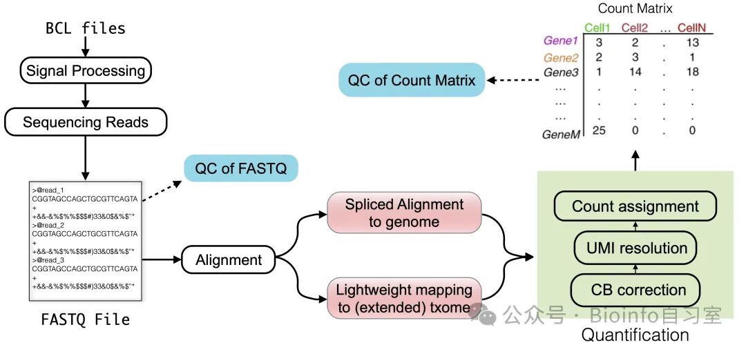
Figure 1. Overview of this chapter. This section focuses on the "Quantification" step in the lower right.
01
Cell Barcode Correction
In recent years, droplet-based single-cell isolation technologies — such as those offered by 10x Genomics — have become indispensable tools for studying the origins and consequences of cellular heterogeneity. In these systems, the RNA from each captured cell is encapsulated inside a water-in-oil droplet together with a uniquely barcoded gel bead. The bead tags each cell's RNA with a short, unique nucleotide sequence called a cell barcode (CB). These barcodes are subsequently sequenced alongside the cDNA fragments reverse-transcribed from the RNA. Thanks to the high diversity of bead-associated barcodes, the sequencing data can be computationally demultiplexed into individual "cell bins" for downstream analysis.
The Effect of Alignment Orientation
Depending on the library chemistry and user-defined processing options, not all reads aligned to the reference genome are used for quantification and barcode correction. One common filter is alignment strand orientation: certain library protocols require that aligned reads originate from a specific strand of the transcript. For example, in the 10x Genomics 3′ Chromium chemistry, reads from genuine captured RNA should align to the forward (sense) strand of the transcript — though antisense reads do also arise during alignment. Researchers may choose to discard or filter reads aligning in the reverse-complement orientation. If a strand-specific protocol is used, this should be explicitly documented. Note: bulk RNA-seq paired-end libraries are typically strand-specific and align to the reverse strand.
Key Challenges in Barcode Correction
Despite the power of barcode technology, errors in practice can cause the observed number of unique cell barcodes to diverge from the true number of captured cells. Common sources of discrepancy include:
- Doublets/multiplets: A single droplet occasionally captures two or more cells sharing the same barcode, leading to an underestimate of cell count.
- Empty droplets: Some droplets contain no cell, yet ambient RNA is still tagged and sequenced, inflating the apparent cell count.
- Sequencing errors: PCR amplification or sequencing can introduce base substitutions in the barcode sequence, further distorting cell count estimates.
To address these issues, a variety of computational tools have been developed to filter low-quality data and correct barcode errors, including:
- Ambient RNA removal: Algorithms to identify and subtract non-specific RNA signals from the background.
- Doublet detection: Statistical models to flag barcodes likely representing two cells.
- Sequencing error correction: Correcting small errors during sequencing based on barcode sequence similarity.
Common Correction Strategies
Whitelist-based correction:
Technologies such as 10x Genomics use a predefined list of valid barcodes (commonly called a "whitelist"). If an observed barcode is sufficiently close to a whitelist entry — for example, differing by only a single base — it is corrected to that whitelist sequence. This approach is efficient, but ambiguity can arise when a barcode is equidistant from multiple whitelist entries.
Note: Barcode similarity is measured using Hamming distance (the number of positions at which two equal-length strings differ) or edit distance / Levenshtein distance (the minimum number of single-character edits required to transform one string into another).
Knee-point / inflection-point method:
When no whitelist is available, a barcode frequency distribution plot can be used to identify a characteristic "knee" or "elbow" point that separates high-quality (cell-associated) barcodes from low-quality (empty droplet) barcodes. This approach is flexible and applicable across a wide range of experimental conditions, though it can be less robust in some situations.
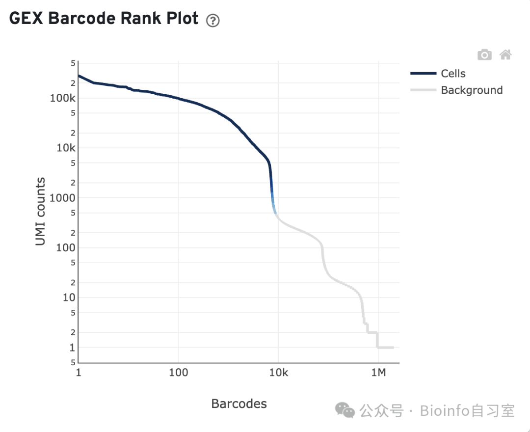
Figure 2. Illustration of a barcode frequency distribution. Cell Ranger identifies the "knee point" to distinguish cell-containing barcodes from background.
Expected cell count filtering:
Users can supply an expected cell count; the algorithm then ranks barcodes by frequency and selects the top candidates most likely to represent true cells.
Hard threshold filtering:
The simplest approach is to set a frequency threshold directly, treating all barcodes above the cutoff as valid. This method requires good prior knowledge of the experimental data.
Determining which observed barcodes represent true cells remains an active research problem, and single-cell versus single-nucleus experiments each introduce their own complications. Moreover, as single-cell sequencing scales up, the limited diversity of barcode sequences may lead to collision conflicts during correction. Addressing these issues will require smarter barcode design strategies and longer nucleotide sequences.
02
UMI Resolution and Quantification
After cell barcode correction, the next task is to quantify gene expression in each cell. This relies on unique molecular identifiers (UMIs), short random sequences added to each cDNA molecule during reverse transcription to tag individual pre-amplification RNA molecules, enabling accurate estimation of true transcript abundance.
Under ideal conditions:
- Every read carries the correct UMI,
- All reads with the same UMI align uniquely to the same gene,
- And each UMI corresponds one-to-one with a pre-PCR mRNA molecule.
In this ideal scenario, deduplication is straightforward: all reads sharing a UMI are PCR duplicates of the same original molecule, so the molecular count for a gene in a cell is simply the number of distinct UMIs. In practice, however, two key complications make simple deduplication insufficient:
UMI errors: During PCR amplification or sequencing, a UMI may acquire a mutation or be miscalled. If left uncorrected, this inflates the estimated number of RNA molecules.
Multimapping: Some UMIs map to multiple genes, making it impossible to determine their true origin. Simply discarding these reads can introduce bias or information loss.
Additional complications include:
Convergent collisions: The same UMI sequence is used to label two different original molecules from the same gene in the same cell. This is relatively rare and has a minor effect on results.
Divergent collisions: A single original molecule gives rise to multiple different UMIs at different positions. This issue is particularly prevalent when working with intronic reads from unspliced transcripts, and remains an active area of research.
Given the widespread use of UMIs in high-throughput single-cell RNA sequencing, accurately estimating gene abundance by resolving these ambiguities has attracted considerable attention, spawning multiple UMI resolution methodologies.
Graph-Based UMI Resolution
To address the challenges above, graph-based UMI resolution methods have been developed. These represent UMIs and their mapping relationships as a UMI graph, then progressively simplify the graph to derive true per-gene molecular counts. (Note: the original text contains substantial mathematical detail; here we provide a high-level summary of the main steps.)
1. Define nodes:
Each node represents a group of reads sharing the same UMI and mapping information. Specifically, if two reads have identical UMI tags and map to the same reference locus or gene, they belong to the same node. If a UMI maps to multiple genes, that node is called a multigene node and requires further handling.
2. Define edges:
An edge is drawn between two nodes if their UMI sequences are very similar (e.g., differ by only one base). Formally, edges are defined based on:
- UMI sequence similarity: Hamming distance or edit distance (see above). If two UMIs are within a specified distance threshold (e.g., 1), they are assumed to potentially derive from the same original molecule.
- Mapping intersection: If two nodes share at least one gene in their mapping sets, an edge connects them.
3. Simplify the graph:
The graph is iteratively simplified by merging similar nodes or removing redundant edges until each remaining node corresponds to a unique original RNA molecule. Common approaches include:
- Connected components: Partitioning the graph into connected components, each representing one original molecule.
- Greedy collapsing: Iteratively merging similar nodes until a stopping criterion is met.
- Arborescence search: Identifying rule-compliant subgraphs (e.g., monochromatic spanning trees) to reduce graph complexity.
Handling and Quantifying Multigene UMIs
Multigene UMIs, as the name implies, are UMIs that map to multiple genes. Their presence introduces uncertainty in gene expression quantification. Two main approaches have been proposed:
(1) Discard
The simplest solution is to discard all multigene UMIs. However, this inevitably leads to data loss, particularly for gene families with high sequence similarity that naturally generate more multimapping reads.
(2) Probabilistic assignment
More sophisticated methods use statistical models — most notably the Expectation-Maximization (EM) algorithm — to probabilistically assign multigene UMIs to their most likely gene of origin.
The EM algorithm is an iterative optimization method for estimating the distribution of latent variables. Applied to UMI resolution, the steps are:
- Initialize gene expression estimates.
- Using the current estimates, calculate the probability that each multigene UMI belongs to each candidate gene.
- Update the gene expression estimates.
- Repeat until convergence.
This approach maximizes the use of available information and avoids the systematic bias introduced by simple discarding. Since each cell provides limited data in a single-cell experiment, analyzing cells in isolation can yield imprecise estimates. Recent methods have therefore proposed cross-cell information sharing to improve UMI resolution and quantification of lowly expressed genes. The final output is a per-cell gene count matrix — the raw expression data that feeds into all downstream analyses.
03
Closing Thoughts
The incredibly dense third chapter of the original book is nearly complete! Because this chapter contains so many technical details and mathematical models, quite a bit of simplification and restructuring was involved in writing these notes (while preserving all the key concepts and frameworks). I hope readers haven't found it too daunting. Starting from the next chapter, we'll enter the world of downstream analysis — the part that most researchers are most eager to get into. Before diving into hands-on data analysis, the book introduces the Python/scanpy-based analysis framework and its ecosystem tools, as well as interoperability between the major analysis ecosystems (SingleCellExperiment, Seurat, and more). Stay tuned if you're looking to get started with the scanpy ecosystem!
Next preview: Quality control strategies for count matrices (overview). Don't miss it!
Originally posted on WeChat Official Account: bioinfo_studyroom