Single-Cell Best Practices

Quality Control

SECTION PREVIEW

1. Understand common QC metrics and thresholds; learn to plot QC figures to assess data quality

2. Use SoupX to remove ambient RNA contamination

3. Use scDblFinder for doublet detection and understand how doublet detection works

Corresponding to Chapter 6 (Quality Control) of the original text

Single-cell RNA sequencing data has two important characteristics: first, due to mRNA capture limitations, the data contains abundant zero values (dropout events); second, the ability to correct for and control data quality is limited, because technical artifacts may be confounded with biological effects. We must therefore choose preprocessing methods suited to the nature of scRNA-seq data, so as not to over-correct or inadvertently remove genuine biological signal.

As sequencing technology has advanced and cell-capture throughput has increased, single-cell analysis tools have evolved rapidly. Many tools are now dedicated to preprocessing steps, including: doublet detection, quality control, normalization, feature selection, and dimensionality reduction. The choice of tools significantly affects downstream analysis and interpretation. Over-filtering can cause the loss of rare cell subpopulations, while overly permissive filtering can compromise the accuracy of cell annotation. Selecting validated, best-practice tools is therefore essential.

In this tutorial, we start from single-cell data that has already been through upstream processing (a UMI count matrix), i.e., a matrix of dimensions barcodes × transcripts. We use "barcodes" rather than "cells" here, because a barcode may tag multiple cells (a doublet) or no cell at all (an empty droplet).

01

Environment Setup and Data Preparation

We use the 10x Multiome dataset from the 2021 NeurIPS single-cell data integration challenge. This dataset contains bone marrow mononuclear cells from 12 healthy human donors, measured at four different sites, producing nested batch effects. This tutorial uses donor 8, sample 4 to demonstrate the preprocessing workflow (see the end of this article for instructions on obtaining the example data).

import numpy as np
import scanpy as sc
import seaborn as sns
from scipy.stats import median_abs_deviation

sc.settings.verbosity = 0
sc.settings.set_figure_params(dpi=80, facecolor="white", frameon=False)

# Load data
adata = sc.read_10x_h5(
    filename="filtered_feature_bc_matrix.h5",
    backup_url="https://figshare.com/ndownloader/files/39546196",
)

After loading the data, scanpy will warn that variable names are not unique. We run var_names_make_unique() to append a numeric suffix to duplicate gene names.

Note: Other common approaches for handling duplicate genes include: 1. keeping only the first occurrence or the one with the highest count, and 2. summing the counts of all duplicate genes. Each approach has trade-offs; choose based on your needs.

adata.var_names_make_unique()

This dataset contains 16,934 barcodes and 36,601 genes. The per-gene (column) annotation .var also includes genome, gene_ids (Ensembl IDs), and feature_types.

Most downstream analyses assume that each observation represents a single, intact cell. However, low-quality cells, ambient RNA contamination, and doublets can all violate this assumption. Quality control should therefore be performed before any downstream analysis.

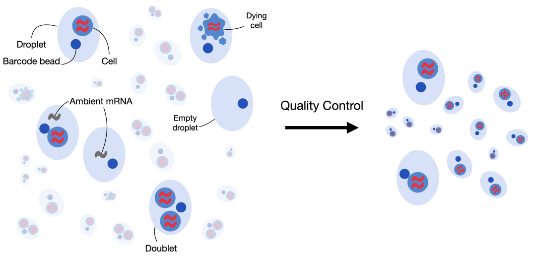Sources of noise in single-cell data (source: scbp)

02

Filtering Low-Quality Cells

Key Metrics

Cell-level quality control is based on three key covariates:

1. 1. Number of counts per barcode (library size / sequencing depth)
2. 2. Number of genes detected per barcode
3. 3. Fraction of counts from mitochondrial genes per barcode

Low gene counts, low sequencing depth, and a high mitochondrial fraction may all indicate a damaged cell membrane and warrant filtering. However, these metrics must be interpreted in combination: cells with a high mitochondrial fraction may genuinely be engaged in respiratory processes; cells with unusually low or high counts may correspond to quiescent or physically large cells, respectively. A lenient filtering strategy is recommended to avoid discarding rare but biologically important subpopulations.

Automated Threshold Setting

Traditionally, researchers have manually set thresholds for these metrics — for example, requiring at least 500 genes detected or a mitochondrial fraction below 10%. Although fixed thresholds generally have a modest effect on downstream analysis, they may not generalize to certain disease contexts or tissue types. For instance, mitochondrial gene content may be broadly elevated in tumour cells, and some quiescent cell types may express relatively few genes overall.

Moreover, data quality can vary across experiments depending on the library preparation method and sequencing platform. When working with many samples or datasets, manually setting thresholds is both time-consuming and error-prone.

We therefore recommend using the median absolute deviation (MAD) to set thresholds automatically:

A starting point of 5 MADs is typically used as a lenient filtering strategy. It is worth emphasising that QC is not a one-and-done step — thresholds are often revisited and refined at later stages such as annotation.

adata.var["mt"] = adata.var_names.str.startswith("MT-")  # mitochondrial genes
adata.var["ribo"] = adata.var_names.str.startswith(("RPS", "RPL"))  # ribosomal genes
adata.var["hb"] = adata.var_names.str.contains("^HB[^(P)]")  # hemoglobin genes

Calculate QC metrics:

sc.pp.calculate_qc_metrics(
    adata, qc_vars=["mt", "ribo", "hb"], inplace=True, percent_top=[20], log1p=True
)

Key output metrics:

• • n_genes_by_counts: Number of genes with at least one count in the cell
• • total_counts: Total UMI count per cell (library size)
• • pct_counts_mt: Percentage of counts from mitochondrial genes

QC Plots

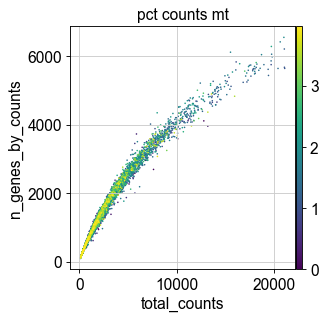
Plot the three QC variables: n_genes_by_counts, total_counts, and pct_counts_mt.

p1 = sns.displot(adata.obs["total_counts"], bins=100, kde=False)
# sc.pl.violin(adata, 'total_counts')
p2 = sc.pl.violin(adata, "pct_counts_mt")
p3 = sc.pl.scatter(adata, "total_counts", "n_genes_by_counts", color="pct_counts_mt")

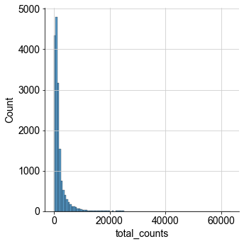
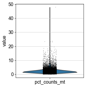
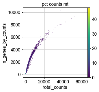
From the plots, some cells show a relatively high mitochondrial count percentage (typically associated with cell degradation), but the majority have mitochondrial fractions below 20% (a commonly used rule-of-thumb threshold). We now apply MAD-based automated filtering:

# Define outlier filter function
def is_outlier(adata, metric: str, nmads: int):
    M = adata.obs[metric]
    outlier = (M < np.median(M) - nmads * median_abs_deviation(M)) | (
        np.median(M) + nmads * median_abs_deviation(M) < M
    )
    return outlier

# Apply 5 MAD threshold
adata.obs["outlier"] = (
    is_outlier(adata, "log1p_total_counts", 5)
    | is_outlier(adata, "log1p_n_genes_by_counts", 5)
    | is_outlier(adata, "pct_counts_in_top_20_genes", 5)
)

# Mitochondrial genes: 3 MADs plus a hard cutoff of 8%
adata.obs["mt_outlier"] = is_outlier(adata, "pct_counts_mt", 3) | (
    adata.obs["pct_counts_mt"] > 8
)

# Check cell count before and after filtering
print(f"Total number of cells: {adata.n_obs}")
adata = adata[(~adata.obs.outlier) & (~adata.obs.mt_outlier)].copy()

print(f"Number of cells after filtering of low quality cells: {adata.n_obs}")
# Total number of cells: 16934
# Number of cells after filtering of low quality cells: 14814

Post-QC check:

p1 = sc.pl.scatter(adata, "total_counts", "n_genes_by_counts", color="pct_counts_mt")

03

Ambient RNA Removal

In droplet-based technologies, ambient RNA contamination is a common artefact. Free-floating mRNA released from lysed cells is captured alongside cellular mRNA and sequenced together — forming what is known as the "soup".

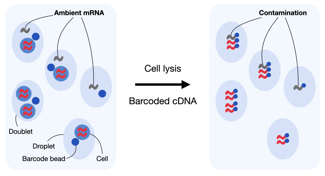Ambient RNA contamination (source: scbp)

Correction with SoupX

SoupX is the leading tool for ambient RNA correction. Its workflow consists of three steps:

1. 1. Estimating the soup profile: Infer the ambient mRNA expression profile from empty droplets.
2. 2. Estimating the contamination fraction: Calculate the cell-specific contamination fraction.
3. 3. Correcting the count matrix: Adjust the count matrix based on the ambient expression profile and the estimated contamination.

First, load the necessary libraries:

import logging

import anndata2ri
import rpy2.rinterface_lib.callbacks as rcb
import rpy2.robjects as ro

rcb.logger.setLevel(logging.ERROR)
ro.pandas2ri.activate()
anndata2ri.activate()

%load_ext rpy2.ipython

%%R
library(SoupX)

SoupX can be run without clustering information, but providing a rough clustering improves results. It is compatible with the default clusters produced by Cell Ranger, or you can supply manually defined clusters.

Perform a quick PCA and Leiden clustering:

# Create a copy
adata_pp = adata.copy()
# Normalize
sc.pp.normalize_per_cell(adata_pp)
sc.pp.log1p(adata_pp)
# PCA, neighbors, dimensionality reduction
sc.pp.pca(adata_pp)
sc.pp.neighbors(adata_pp)
sc.tl.leiden(adata_pp, key_added="soupx_groups")

# Export clustering results as a vector
soupx_groups = adata_pp.obs["soupx_groups"]
# Delete copy to save memory
del adata_pp

# Export cell names, gene names, and the filtered feature x barcode matrix (transpose!)
cells = adata.obs_names
genes = adata.var_names
data = adata.X.T

In addition to the filtered count matrix (filtered_feature_bc_matrix) used for standard analysis, SoupX also requires the original, unfiltered Cell Ranger output matrix (raw_feature_bc_matrix). The latter contains information from empty droplets, which SoupX uses to estimate the ambient signal.

adata_raw = sc.read_10x_h5(
    filename="raw_feature_bc_matrix.h5",
    backup_url="https://figshare.com/ndownloader/files/39546217",
)
adata_raw.var_names_make_unique()
# Export unfiltered matrix
data_tod = adata_raw.X.T
# Can be deleted now
del adata_raw

Now run SoupX:

%%R -i data -i data_tod -i genes -i cells -i soupx_groups -o out
# Set row and column names
rownames(data) = genes
colnames(data) = cells
# Ensure correct sparse format for count and droplet tables
data <- as(data, "sparseMatrix")
data_tod <- as(data_tod, "sparseMatrix")

# Create SoupChannel object for SoupX
sc = SoupChannel(data_tod, data, calcSoupProfile = FALSE)

# Add additional metadata to the SoupChannel object
soupProf = data.frame(row.names = rownames(data), est = rowSums(data)/sum(data), counts = rowSums(data))
sc = setSoupProfile(sc, soupProf)
# Set clustering information in SoupChannel
sc = setClusters(sc, soupx_groups)

# Estimate contamination fraction
sc  = autoEstCont(sc, doPlot=FALSE)
# Infer corrected count table and round to integers
out = adjustCounts(sc, roundToInt = TRUE)

Import the corrected matrix back into AnnData:

adata.layers["counts"] = adata.X
adata.layers["soupX_counts"] = out.T
adata.X = adata.layers["soupX_counts"]

Next, filter out genes not detected in at least 20 cells, as these genes provide no useful information.

print(f"Total number of genes: {adata.n_vars}")

# At least 20 cells - filter out zero-count genes
sc.pp.filter_genes(adata, min_cells=20)
print(f"Number of genes after cell filtering: {adata.n_vars}")
# Total number of genes: 36601
# Number of genes after cell filter: 20171

04

Doublet Removal

Types of Doublets

A doublet is defined as two cells that are sequenced under the same cell barcode — for example, when they are captured in the same droplet. If a doublet is formed from the same cell type (but from different individuals), it is called homotypic; otherwise, it is called heterotypic.

Homotypic doublets are not necessarily identifiable from the count matrix alone, but are generally considered less harmful because they can often be resolved through cell hashing or SNP-based demultiplexing. Their detection is therefore not the primary goal of doublet-detection methods.

Heterotypic doublets — formed from cells of different types or states — are the main target of doublet detection. They are likely to be misclassified during annotation, which can seriously distort downstream analysis. They must therefore be identified and removed during preprocessing.

Doublets can be detected by their elevated count numbers and transcriptomic signatures, or by generating artificial doublets and comparing them to observed cells in the dataset. This tutorial demonstrates the R package scDblFinder, which achieves the highest doublet-detection accuracy in benchmark comparisons while also offering excellent computational efficiency and stability (Xi and Li, 2021).

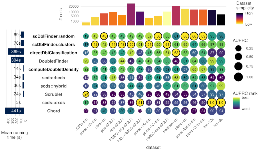Benchmark results, Xi and Li, 2021

scDblFinder

scDblFinder detects doublets through the following steps:

1. 1. Randomly select pairs of droplets and create artificial doublets by averaging their gene expression profiles.
2. 2. Construct a k-nearest neighbour (kNN) graph of each droplet in PCA space.
3. 3. The doublet score is defined as the proportion of artificial doublets among the k nearest neighbours of each cell.

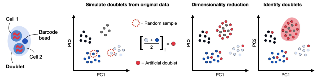How scDblFinder works (source: scbp)

%%R
library(Seurat)
library(scater)
library(scDblFinder)
library(BiocParallel)

# Export expression matrix
data_mat = adata.X.T

The input and output of scDblFinder are both SingleCellExperiment objects. Doublet-related results are stored in the object's metadata:

• • sce$scDblFinder.score: Final doublet score (higher values indicate a greater likelihood of being a doublet)

• • sce$scDblFinder.ratio: Proportion of artificial doublets in the cell's neighbourhood

• • sce$scDblFinder.class: Classification result (singlet or doublet)

  %%R -i data_mat -o doublet_score -o doublet_class

  set.seed(123)
  sce = scDblFinder(
  SingleCellExperiment(
  list(counts=data_mat),
  )
  )

  Export scores and classification results

  doublet_score = sce$scDblFinder.score
  doublet_class = sce$scDblFinder.class

Add the results to the AnnData object:

adata.obs["scDblFinder_score"] = doublet_score
adata.obs["scDblFinder_class"] = doublet_class
adata.obs.scDblFinder_class.value_counts()
# singlet    11956
# doublet     2858
# Name: scDblFinder_class, dtype: int64

# Save QC-processed data
adata.write("s4d8_quality_control.h5ad")

It is recommended to retain the detected doublets for now and evaluate them further during the visualisation and clustering steps.

05

Closing Thoughts

We've made it through the QC section — have you got a clear picture of the steps and their order? Here's a summary of the key takeaways:

1. Quality control is a foundational step in single-cell analysis. The right strategy ensures data quality while preserving important biological signals. Filtering parameters can and should be re-evaluated and adjusted in light of results from subsequent steps such as clustering.

2. Use MAD-based automated thresholds for initial filtering, setting lenient cutoffs to avoid inadvertently discarding small subpopulations. In terms of priority: cell-level filtering > gene-level filtering.

3. The basic order is: low-quality cells → ambient RNA → doublets. Doublet filtering need not be finalised in a single pass — repeated rounds of dimensionality reduction and clustering can help you evaluate and refine the results.

---

Originally posted on WeChat Official Account: bioinfo_studyroom