Learn Single-Cell Analysis with Theis Lab: Tracing the \"Fate\" Trajectory of Cells

Single-Cell Best Practices
Pseudotime
SECTION PREVIEW
What is "pseudotime"? How is it constructed from seemingly disordered "snapshots"?
Graph methods, probabilistic methods... What are the differences in the logic behind various Trajectory Inference (TI) algorithms?
Root Cell: Why is "choosing the right starting point" the most critical step in pseudotime analysis?
Hands-on practice: Both DPT and Palantir are well-known tools — how do we compare and select the more reliable pseudotime result?
This section corresponds to Chapter 13 Pseudotemporal ordering in the original book.
Single-cell sequencing technologies (such as scRNA-seq) provide us with an unprecedented resolution for measuring biological tissues. These technologies can therefore help us "decode" and understand cellular heterogeneity and the dynamics of biological processes.
However, classical scRNA-seq protocols destroy cells during sequencing, which means we cannot track how a single cell's gene expression profile changes over time. Although recent advances (such as Live-seq) allow continuous transcriptome recording, they remain experimentally challenging and currently difficult to scale to large datasets.
We must therefore infer the underlying dynamic processes from the "snapshot" data obtained by sequencing.
What Is Pseudotime?
You might ask: if the data is a snapshot from a single time point, how can we infer anything dynamic?
The key lies in the asynchronous nature of biological processes. Even when a sample is collected at a single experimental time point, we observe many different cell types. This is because cells do not develop in synchrony — a single-time-point "snapshot" therefore captures cells at a range of different developmental stages (for example, from stem cells to progenitors and on to terminally differentiated cells).
The field of Trajectory Inference (TI) aims to reconstruct this developmental "landscape" by ordering the observed cell states along a developmental continuum.
This process maps discrete cell annotations (such as "stem cell" or "progenitor") onto a continuous axis — and this continuous value is called pseudotime.
- Pseudotime orders cells according to their relative stage in a developmental process.
- Immature cells are assigned small pseudotime values, while mature cells receive larger values.
- For example, when studying a bone marrow sample, haematopoietic stem cells (HSCs) would receive low pseudotime values, while erythroid cells would receive high values.
- In scRNA-seq data, this ordering is based on the transcriptomic profiles of the cells.
- Crucially: constructing pseudotime typically requires specifying an initial cell or root cell — the starting point of the entire trajectory.
How Is Pseudotime Constructed?
Pseudotime construction generally follows a common workflow:
- Dimensionality reduction: The ultra-high-dimensional single-cell data is first projected into a low-dimensional representation, since dynamic processes typically unfold on a low-dimensional manifold. Dimensionality reduction may rely on principal components (PCA, e.g. Palantir) or diffusion components (e.g. DPT).
- Trajectory construction: In the low-dimensional space, pseudotime is constructed using one of several main strategies.
1. Cluster-Based Approach
Cells are first clustered, and then connections between clusters are identified. Pseudotime is constructed by ordering the clusters — often using a minimum spanning tree (MST) to link them.
2. Graph-Based Approach
Connections between cells in the low-dimensional space are found first, defining a graph. Clusters and ordering are then defined based on this graph. For example, PAGA partitions the graph into Leiden clusters and estimates the connectivity between them. This approach preserves the global topological structure of the data and is computationally efficient.
3. Manifold Learning Approach
Similar to the cluster-based approach, but this method uses principal curves or graphs to estimate the underlying trajectory, thereby defining inter-cluster connections. Slingshot is a well-known representative of this approach.
4. Probabilistic Frameworks
This approach assigns transition probabilities to ordered cell pairs, quantifying the likelihood that one cell is an ancestor of another.
- DPT (Diffusion Pseudotime) defines pseudotime as the difference between consecutive states in a random walk.
- Palantir models the trajectory itself as a Markov chain.
- Both methods rely on probabilistic frameworks and both require a root cell to be specified, relative to which pseudotime is calculated.
★
Editor's note: How do you choose a method?
Trajectory inference is a well-studied field with many methods available. Selecting the right method requires some prior knowledge of the biology at hand. You need to know, for example, whether the process is linear, cyclic, or branching. Different TI methods are designed for different trajectory topologies. If you are uncertain, dynguidelines provides a comprehensive overview of available algorithms and their properties to help guide your selection.
 A preview of the dynguidelines interface
What Comes After Pseudotime?
TI and pseudotime are themselves valuable, but they typically serve as a stepping stone to more refined analyses. Based on TI and pseudotime, we can investigate classical biological questions such as:
- Identifying terminal states.
- Identifying lineage bifurcations.
- Characterising genes that drive fate decisions.
For example, Palantir identifies terminal states by recognising the absorbing states of its Markov chain.
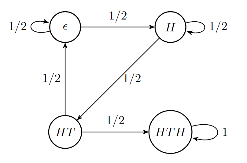 A simple Markov chain: circles represent "states"; numbers/arrows represent transition probabilities between states. The "HTH" state has no outgoing arrows and is therefore an "absorbing state". Source: Wikipedia
As sequencing technology advances, new data modalities (such as ATAC-seq and CITE-seq) and new strategies (such as RNA velocity) are being integrated into TI, enabling future tools to estimate trajectories with greater accuracy and robustness.
Hands-On: Pseudotime Inference in Adult Bone Marrow
Below, we use an adult bone marrow dataset to demonstrate how to construct and compare different pseudotime orderings.
Environment Setup and Data Loading
import scanpy as sc
import pandas as pd
from pathlib import Path

# Set data directory
DATA_DIR = Path("../../data/")
DATA_DIR.mkdir(parents=True, exist_ok=True)

# Define filename
FILE_NAME = DATA_DIR / "bone_marrow.h5ad"

# Load data; if not available locally, download from URL
adata = sc.read(
    filename=FILE_NAME,
    backup_url="https://figshare.com/ndownloader/files/35826944",
)

# Inspect the AnnData object
print(adata)
Output:
AnnData object with n_obs × n_vars = 5780 × 27876
    obs: 'clusters', 'palantir_pseudotime', 'palantir_diff_potential'
    var: 'palantir'
    uns: 'clusters_colors', 'palantir_branch_probs_cell_types'
    obsm: 'MAGIC_imputed_data', 'X_tsne', 'palantir_branch_probs'
    layers: 'spliced', 'unspliced'
Data Preprocessing
The data must be preprocessed before pseudotime can be computed. "Preprocessing" here refers to the standard steps covered in earlier chapters: filtering lowly-expressed genes, normalisation, log-transformation, highly variable gene selection, dimensionality reduction, and kNN graph construction.
# 1. Filter: remove genes expressed in fewer than 20 cells
sc.pp.filter_genes(adata, min_counts=20)

# 2. Normalise: normalise cell size (normalize total)
sc.pp.normalize_total(adata)

# 3. Transform: log1p transformation to reduce the effect of outliers
sc.pp.log1p(adata)

# 4. Select: identify highly variable genes
sc.pp.highly_variable_genes(adata)

# 5. Reduce dimensionality: PCA
sc.tl.pca(adata)

# 6. Build graph: construct kNN graph using 10 PCs
sc.pp.neighbors(adata, n_pcs=10)

# Plot t-SNE scatter plot, coloured by 'clusters'
sc.pl.scatter(adata, basis="tsne", color="clusters")
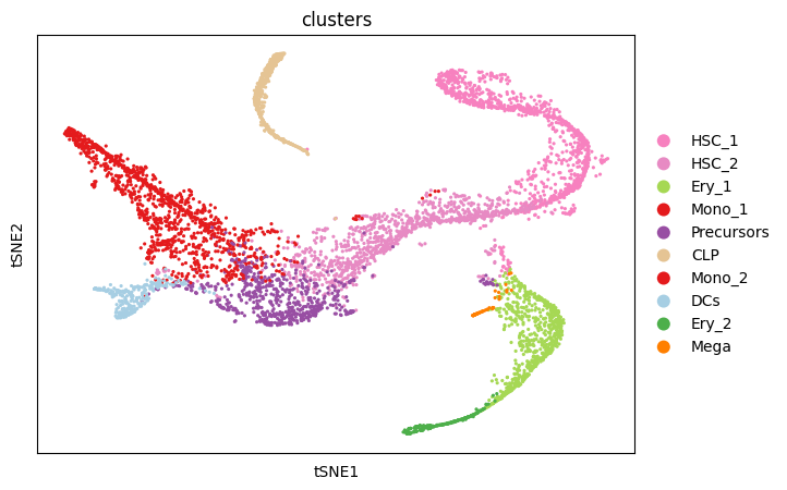
The cell types cluster cleanly together, and the hierarchical structure of haematopoietic development is clearly visible.
Computing Diffusion Pseudotime
Now let's compute Diffusion Pseudotime (DPT).
# 1. Compute diffusion map
sc.tl.diffmap(adata)

# 2. Identify the root cell
# We know that bone marrow differentiation begins from haematopoietic stem cells (HSCs)
# But we don't know which specific cell in the dataset is the starting point
# Strategy: we examine individual diffusion components (DCs),
# and find the stem cell at the extreme end of one dimension (here, DC3)
root_ixs = adata.obsm["X_diffmap"][:, 3].argmin()

# Plot to confirm
sc.pl.scatter(
    adata,
    basis="diffmap",
    color=["clusters"],
    components=[2, 3],
)

# Store the selected root cell index in the AnnData object
adata.uns["iroot"] = root_ixs

# 3. Compute DPT
sc.tl.dpt(adata)
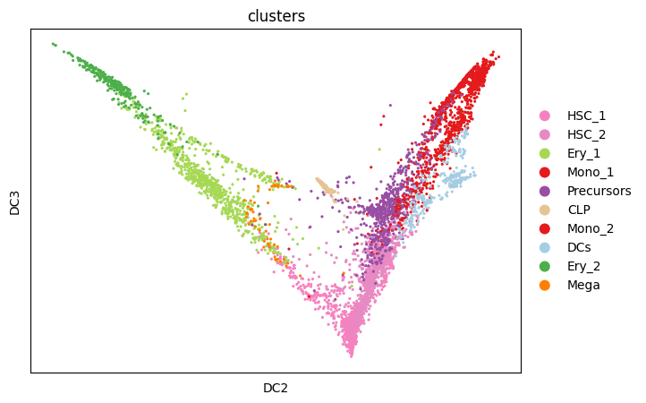
Nearly all TI methods require at least an approximate knowledge of the biological starting point. Selecting the root cell is the most critical — and trickiest — step in pseudotime analysis.
The strategy above is very representative: although we don't know which specific cell is the root, our prior biological knowledge tells us which cell type it belongs to (HSCs). A common approach is therefore to identify the cell within the HSC cluster that sits at the extreme end of a given reduced-dimensional axis (here, the third diffusion component) and designate it as the root cell.
For a more biologically grounded approach to root cell selection, CytoTRACE is a strong option. It predicts the differentiation potential of cells, providing independent support for the developmental ordering implied by pseudotime.
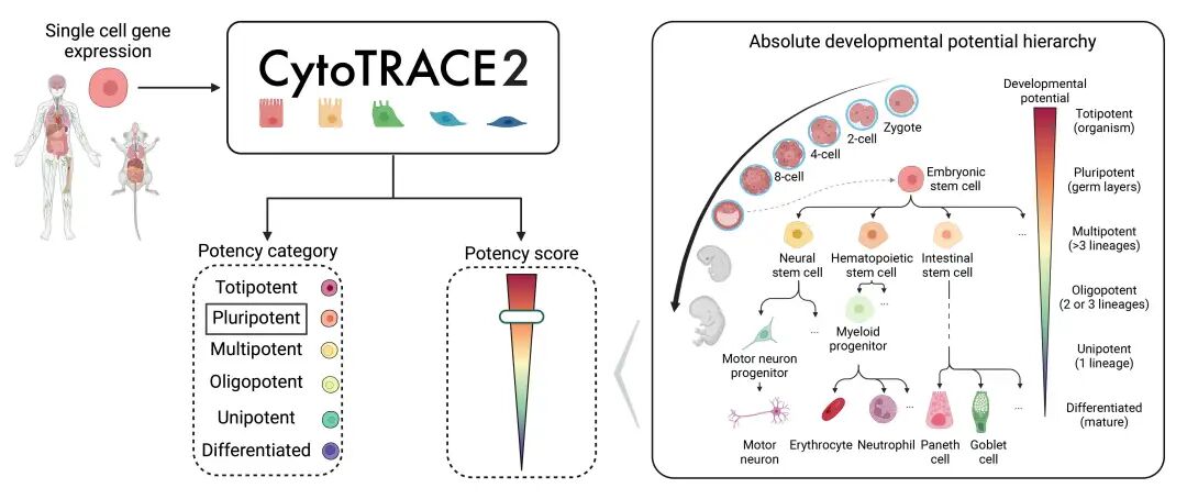 Source: PyPI
Comparing Pseudotime Methods (DPT vs. Palantir)
Different pseudotime methods can give different results. Let's compare the DPT we just computed with the pre-computed Palantir pseudotime already stored in the dataset:
sc.pl.scatter(
    adata,
    basis="tsne",
    color=["dpt_pseudotime", "palantir_pseudotime"],
    color_map="gnuplot2",
)
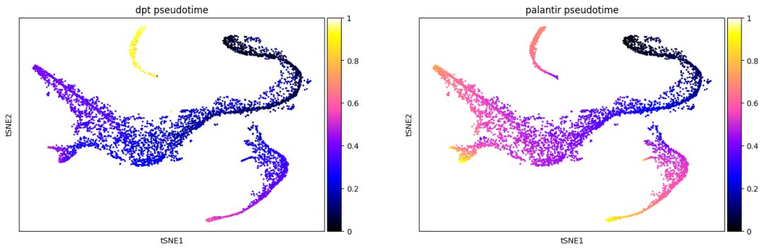
Observations:
DPT: The CLP cluster has anomalously high DPT pseudotime values (yellow), which is inconsistent with biology.
Palantir: Pseudotime values (colour scale) increase continuously with developmental maturity, from HSCs through each lineage.
Let's also visualise the pseudotime distributions per cluster using violin plots:
sc.pl.violin(
    adata,
    keys=["dpt_pseudotime", "palantir_pseudotime"],
    groupby="clusters",
    rotation=45,
    # Ordered by known developmental sequence
    order=[
        "HSC_1",
        "HSC_2",
        "Precursors",
        "Ery_1",
        "Ery_2",
        "Mono_1",
        "Mono_2",
        "CLP",
        "DCs",
        "Mega",
    ],
)
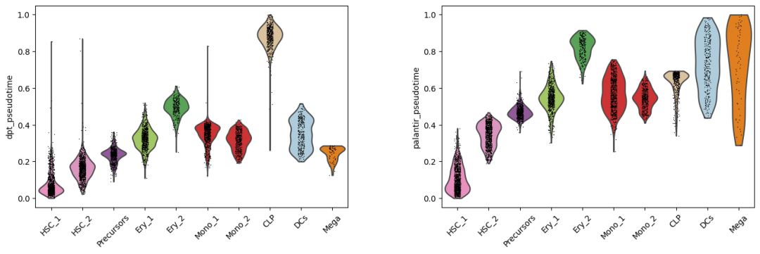
Observations:
DPT: Again, the CLP cluster stands out as an outlier. Additionally, many cells in HSC_1 and HSC_2 — which should be the developmental starting points — carry unexpectedly high pseudotime values, contradicting our prior biological knowledge.
Palantir: The violin plot sequence from HSC_1 to Mega shows a smooth, monotonic increase in pseudotime values, which is consistent with known haematopoietic differentiation.
Conclusion: Given these observations and prior knowledge of bone marrow development, we would choose Palantir for downstream analyses.
Summary and Closing Thoughts
A few key takeaways from this pseudotime chapter:
Prior biological knowledge is required: TI methods such as DPT and Palantir generally need (at least an approximate) specification of the biological starting point — i.e., the root cell.
Match the method to the process: The nature of the biological process (linear, branching, or cyclic) determines which TI algorithm is appropriate.
Use available tools wisely: dynguidelines is an excellent resource for choosing the right TI method based on the characteristics of your data.
In R, popular alternatives include Slingshot and Monocle2/3. Which method do you find the most useful — or the most frustrating? Share your experience in the comments!
Welcome all bioinformatics enthusiasts to join the Bioinfo Study Room community group:

Originally posted on WeChat Official Account: bioinfo_studyroom