Downstream Notes 2: Can You Recover the Original Counts from Normalized Data? Here's the Trick

February 20, 2026 · 5 min read · Analysis Notes

📢 What's in this post:

Practical tricks for figuring out whether a dataset has been normalized

Hands-on code for reverse-engineering raw counts from normalized data

The reverse-engineering logic for different normalization methods

Hey everyone! I'm back with another downstream analysis note! This time I'm sharing a handy trick: how to back-calculate the original count matrix from normalized data. This is especially useful when working with publicly available datasets, where authors sometimes only release the normalized matrix — but you need the raw counts to apply methods like SCTransform for a fresh analysis.

🤔 Why Would You Need to Recover Raw Counts?

Before we dive in, let's talk about why this situation comes up. Normalization is typically the very first step in single-cell RNA-seq analysis. You've likely heard of CPM, CP10K, TPM, and similar concepts — all normalization methods. Normalized data is better suited for downstream analysis because it corrects for differences in sequencing depth across cells.

📌 Key use cases:

You want to re-normalize the data with a different method (e.g., SCTransform instead of log-normalization)

You need to compare raw expression levels across samples or datasets

Certain analyses require raw counts as input (e.g., differential expression analysis)

🔍 How to Tell Whether Data Has Been Normalized

Before attempting to reverse-engineer counts, you first need to determine whether the data you have is normalized — and if so, which method was used. Here are a few practical checks:

1️⃣ Check the order of magnitude

# Raw counts
# counts <- obj[["RNA"]]$counts
# CPM
# normalized <- NormalizeData(obj, normalization.method = "RC", scale.factor = 1e6)[["RNA"]]$data
# log1p(CP10K)
# lognorm <- NormalizeData(obj, normalization.method = "LogNormalize")[["RNA"]]$data

# Raw counts are typically integers ranging from 0 to a few hundred or thousand
> max(counts)
[1] 4838

# CPM/CP10K normalized values typically range from 0 to 1e6
> max(normalized)  # CPM
[1] 727843.1

# Log-normalized values typically don't exceed 20
> max(lognorm)  # log1p(CP10K)
[1] 8.892808

2️⃣ Check the per-cell sum

# Check the total expression across the first few cells
> colSums(counts)[1:5]
1502 2431 1861 1073 2179

> colSums(normalized)[1:5]  # CPM
1e+06 1e+06 1e+06 1e+06 1e+06

> colSums(lognorm)[1:5]  # log1p(CP10K)
1691.305 1512.919 1982.604 1467.348 1828.618

Key signatures:

After CPM normalization, the per-cell sum should be approximately 1×10⁶
After CP10K normalization, the per-cell sum should be approximately 1×10⁴

3️⃣ Check for decimal values

# The presence of many decimal values strongly suggests normalization has been applied
> head(matrix[, 1])
  Gene1    Gene2    Gene3    Gene4    Gene5
0.00000  3.24156  0.12456  1.95632  0.00000

4️⃣ Check the relative expression of housekeeping genes

A particularly useful trick is to look at the relative expression levels of housekeeping genes, especially those with notably different transcript lengths. This is ideal for detecting whether the data has undergone length-aware normalization (such as TPM or RPKM).

A few commonly used housekeeping genes and their approximate lengths:

ACTB (β-actin): ~1.9 kb
GAPDH: ~1.4 kb
RPL13A: ~1.0 kb
SDHA: ~2.3 kb

# Extract housekeeping gene expression values
housekeeping <- lognorm[c("ACTB", "GAPDH", "SDHA"), ]

# Calculate the ACTB/GAPDH ratio
actb_gapdh_ratio <- mean(housekeeping["ACTB", ]) / mean(housekeeping["GAPDH", ])
[1] 1.18  # Consistent with CP10K normalization

Interpretation:

Under CPM/CP10K normalization: ACTB/GAPDH ratio ≈ 1.1
Under TPM/RPKM normalization: ACTB/GAPDH ratio ≈ 0.85 (because gene length is taken into account)
Under TPM/RPKM, the expression of SDHA (the longest gene) will be noticeably lower than under CPM

🔍 Tip: In single-cell data, dropout effects can distort individual cell measurements, so it's better to look at the average across multiple cells. Also note that housekeeping gene expression can vary across tissues and cell types.

💻 Recovering Raw Counts from log1p CP10K Data

Alright, let's get to the code! Suppose we have a log1p CP10K–normalized matrix and want to recover the original counts.

Reverse-engineering steps:

Undo the log1p transformation: exp(x) - 1
Undo the CP10K scaling: multiply by the per-cell total count divided by 10,000
Round to the nearest integer

# Assume the input normalized matrix is called lognorm

# Step 1: Undo the log1p transformation
unlog_mat <- expm1(lognorm)  # equivalent to exp(lognorm) - 1

# Step 2: Helper function to find the minimum non-zero value in a cell
get_min_nonzero <- function(x) {
  min(x[x > 0])
}

# Step 3: For each cell, use the minimum non-zero value as the scaling reference
raw_counts <- apply(unlog_mat, 2, function(x) {
  min_val <- get_min_nonzero(x)
  round(x / min_val)  # Round to integer
})

🔎 Validating the Result

# 1. Check that all values are integers
all(raw_counts == round(raw_counts))  # Should return TRUE

# 2. Re-normalize the recovered counts and check if they match the original normalized data
library(Seurat)
test_obj <- CreateSeuratObject(raw_counts)
test_obj <- NormalizeData(test_obj)

# 3. Plot original vs. re-normalized data
plot(lognorm[, 1],
     test_obj[["RNA"]]@data[, 1],
     xlab = "Original normalized data",
     ylab = "Re-normalized data",
     main = "Comparison of normalization")
abline(0, 1, col = "red")  # Points should fall on this line if the recovery is perfect

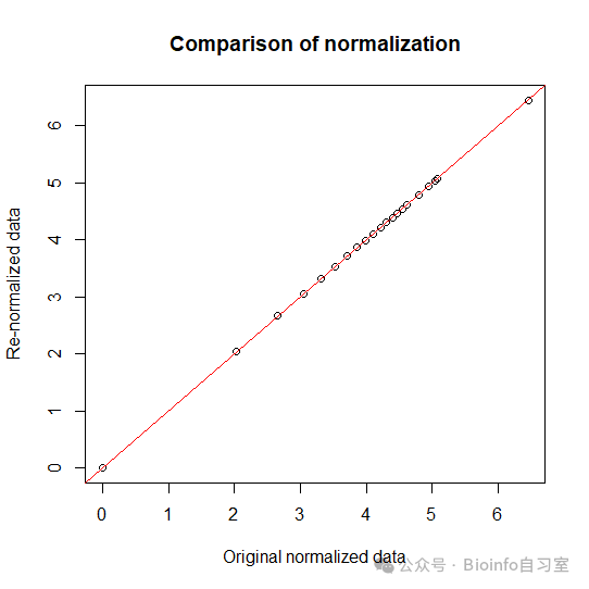
Amazing!

⚠️ Is This Approach Justified?

The core assumption underlying this method is: in UMI-based single-cell data, the minimum non-zero count in any given cell should be 1. This holds for most UMI-based datasets because:

✅ UMI technology enables precise counting of individual transcripts
✅ Counts must be non-negative integers
✅ The smallest possible non-zero count is 1 (a single transcript detected)

⚠️ Caveats:

This method is not universally applicable:

If the original data is not UMI-based (e.g., Smart-seq2), this assumption may not hold

If the data has been normalized with a complex method (e.g., SCTransform), this approach won't work

If data quality is poor (e.g., heavy dropout), the recovered counts may be inaccurate

🔄 Extension: Reversing Other Normalization Methods

The same general logic applies to other normalization methods:

Normalization method	Reverse-engineering approach	Recommended?
log1p CPM	Same as above, using 1×10⁶ instead of 10,000	✅
log2	Apply base-2 exponentiation	✅
TPM	Requires gene length information	❌

📝 Summary

This trick might seem a little "reverse engineering," but it comes in genuinely handy in practice — particularly when working with public datasets or when you want to re-analyze data with a different normalization strategy. That said, keep in mind that any back-calculated count matrix is always an approximation — it can't perfectly reconstruct the original data. Whenever possible, it's always best to obtain and work with the raw count matrix directly!

💌 If you run into issues using this method or have ideas to share, feel free to leave a comment! See you in the next post!

#Bioinformatics #SingleCellSequencing #DataAnalysis #Rlanguage

Originally posted on WeChat Official Account: bioinfo_studyroom

Single Cell Seurat Downstream