Paper Outlook — September 21-27, 2026

· 4 min read · Paper Feed

Paper Outlook — September 21-27, 2026

TL;DR

  • This week highlights how combining molecular layers (DNA methylation, RNA, proteins, spatial maps, and single-cell data) is reshaping our view of cancer and neurodegeneration.
  • Several studies point to the tumor microenvironment, not just the cancer cells themselves, as a driver of disease behavior, drug response, and treatment resistance.
  • Spatial transcriptomics keeps maturing, with new computational methods and practical guides making the technology more accessible to non-specialists.
  • A recurring theme is the discovery of previously hidden biological players, such as small proteins in Alzheimer's brains and rare epigenetic subtypes in pediatric cancers, that could open new diagnostic or therapeutic avenues.

CpG hypermethylation and WNT/AP-1 cooperativity define the epigenetic landscape and a clinical subgroup of high-risk pediatric adrenocortical carcinoma.

Researchers profiled more than 200 rare childhood adrenal cancers using multiple molecular assays together. They identified a high-risk subgroup with distinctive DNA methylation patterns, two active cancer signaling pathways, and poor survival, which could help guide more precise treatment for these children.
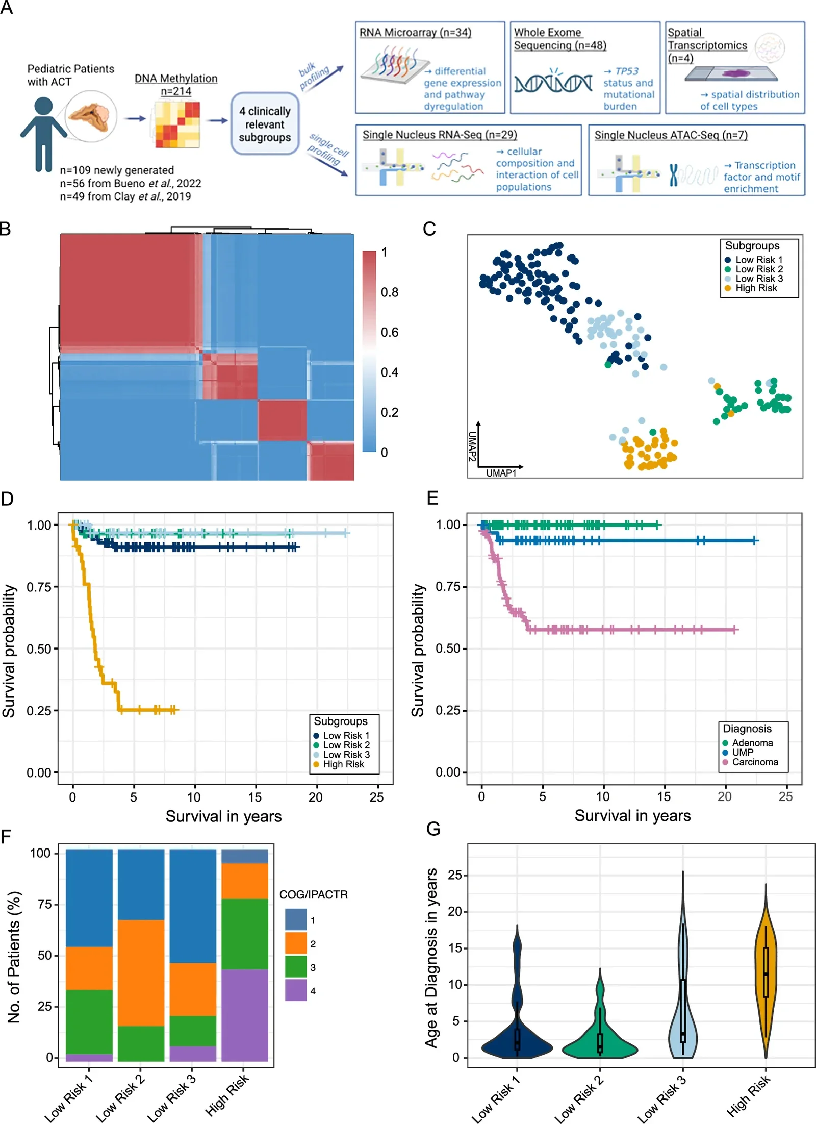
DNA methylation–based stratification of pediatric adrenocortical tumors identifies four clinically distinct subgroups. A Overview of the project presented in this paper. Created in BioRender. Fincke, V. (2026) https://BioRender.com/5ujxlr5 . B Unsupervised clustering of DNA methylation data using Consnsus Clustering identifies four molecular subgroups (Low Risk 1, Low Risk 2, Low Risk 3, and High Risk) in 214 pediatric ACTs. Red indicated samples always cluster together; blue color indicates samples never cluster together (total n = 214; HR, n = 36; LR1, n = 104; LR2, n = 34; LR3, n = 40). C UMAP projection of DNA methylation profiles colored by molecular subgroup (total n = 214; HR, n = 36; LR1, n = 104; LR2, n = 34; LR3, n = 40). D Kaplan–Meier analysis of overall survival across histopathological diagnoses (pACA, n = 82; pACC, n = 92; pUMP, n = 40; log-rank test). E Kaplan–Meier analysis of overall survival across methylation-based subgroups (HR, n = 36; LR1, n = 104; LR2, n = 34; LR3, n = 40; log-rank test). F COG/IPACTR stage at diagnosis across methylation-based subgroups (stage 1, n = 75; stage 2, n = 67; stage 3, n = 27; stage 4, n = 36; stage not available, n = 9; chi-square test). G Age at diagnosis (years) by molecular subgroup (HR, n = 35; LR1, n = 102; LR2, n = 34; LR3, n = 40; age at diagnosis was available for 211 patients). Violin plots show the kernel density distribution of the data; embedded box plots indicate the median (center line), the 25th and 75th percentiles (box bounds), and whiskers extending to the most extreme value within 1.5 × the interquartile range of the box, which define the plotted minima and maxima. Groups were compared by two-sided Kruskal–Wallis test (P = X), followed by two-sided pairwise Dunn’s post hoc tests with Benjamini–Hochberg correction for multiple comparisons. Adjusted P values: LR1 vs LR2, Padj = 0.129; LR1 vs LR3, Padj = 0.018; LR1 vs HR, Padj = X; LR2 vs LR3, Padj = 0.0019; LR2 vs HR, Padj = X; LR3 vs HR, Padj = 1.64 × 10⁻⁴. Source data are provided with this paper.

Fig. 1 from Fincke VE et al., Nature communications (2026). Licensed CC BY. Source: 10.1038/s41467-026-77225-5.

Nature communications (2026)

Read the original → https://doi.org/10.1038/s41467-026-77225-5


A microprotein atlas of the human frontal cortex in Alzheimer's disease.

Scientists built a protein map of the human frontal cortex using Alzheimer's brain tissue, focusing on tiny proteins encoded by small stretches of DNA that are often overlooked. They report over 1,000 of these microproteins, some of which shift in Alzheimer's disease in ways that don't track with known genes, hinting at disease mechanisms that current annotations miss.
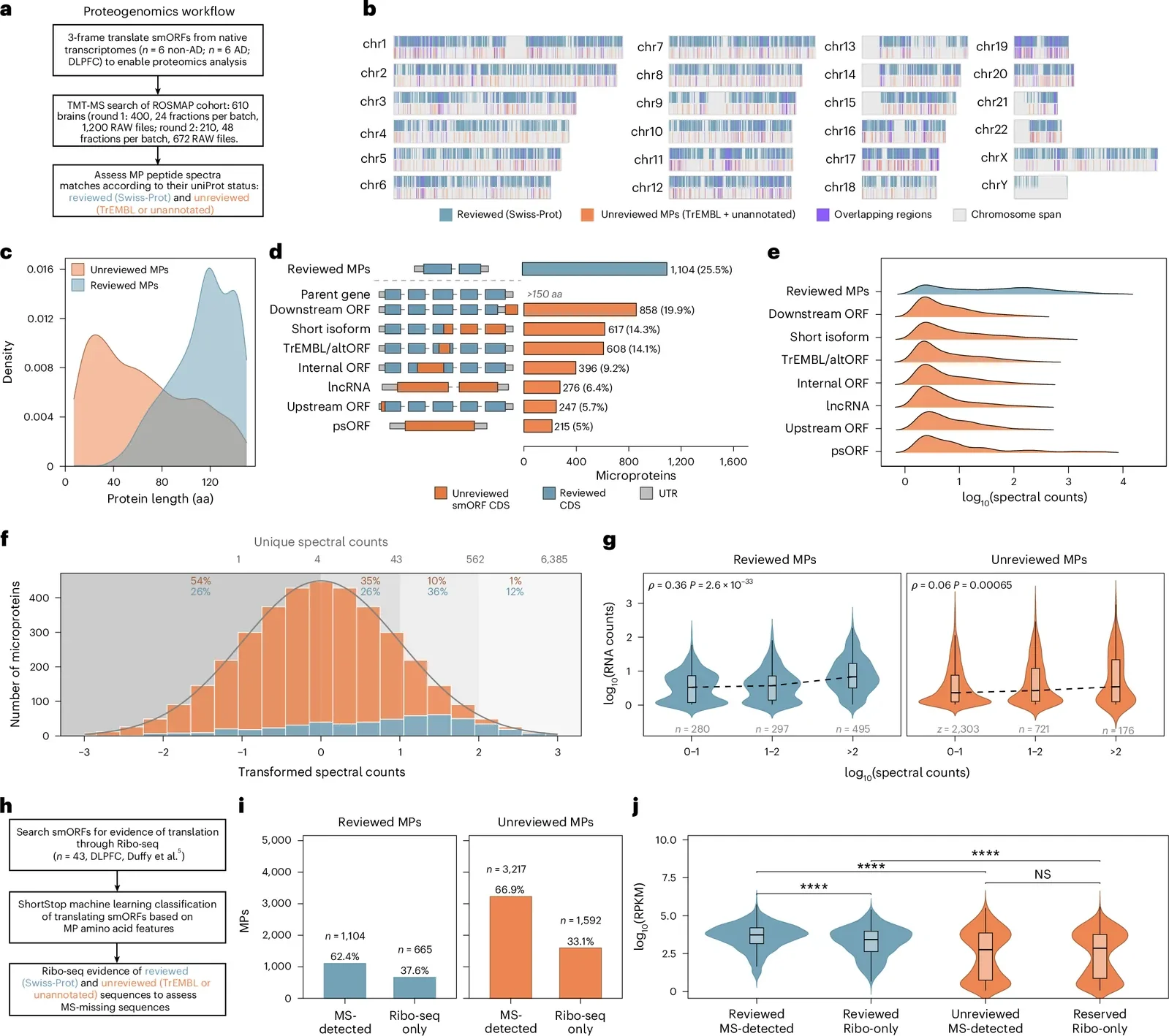
MS evidence of MPs in the aged human frontal cortex. Box plots (embedded within violins where shown): the center line represents the median; the box bounds represent the 25th and 75th percentiles; and the whiskers extend to the most extreme data points within 1.5× the interquartile range (defining the plotted minima and maxima). a , Long-read transcriptomes from 12 DLPFC samples (six AD/six non-AD; six females, six males) were assembled, three-frame translated and appended to the UniProt reference proteome for proteomics search studies. TMT-MS search cohort: 610 brains, biological replicates (round 1: n = 400, 24 fractions per batch, 1,200 RAW files; round 2: n = 210, 48 fractions per batch, 672 RAW files). b , Proteogenomic map of aged human DLPFC according to chromosome: reviewed (Swiss-Prot, teal) and unreviewed (TrEMBL + unannotated, orange) MPs; overlap, purple. c , Protein length density: reviewed ≤150 aa ( n = 1,104) and unreviewed ( n = 3,217) MPs with MS evidence in ROSMAP. d , smORF location and counts ( n = 4,321 total). smORF types are shown according to their position relative to the main ORF of the annotated parental gene (for example, upstream ORF); definitions are given in the Methods . e , Spectral count distribution according to smORF type ( n = 3,732), ridgeline, log 10 scale. f , Total spectral counts ( n = 3,732), reviewed/unreviewed stacked; percentage shown per transformed bin. g , RNA–protein correlation according to the number of spectral count bins (0–1, 1–2, >2). Protein abundance: TMT-MS spectral counts ( n = 610 ROSMAP brains). RNA: counts per million (CPM) ( n = 373 ROSMAP brains). Two-sided Spearman correlation, 95% confidence interval (CI) via Fisher’s z . Reviewed: n = 1,072, ρ = 0.356 (0.302–0.407), P = 2.61 × 10 −33 . Unreviewed: n = 3,200, ρ = 0.060 (0.026–0.095), P = 6.51 × 10 −4 . Correlation was done on razor peptides for Swiss-Prot; correlation was done on unique peptides for unreviewed. h , Ribo-seq (43 non-AD DLPFC brains) recovered MPs missed by MS; ShortStop classified translated smORFs according to aa physicochemical properties. i , MPs according to detection evidence (MS-detected versus Ribo-seq only), reviewed/unreviewed. j , Ribosome occupancy (log 10 reads per kilobase per million mapped reads (RPKM)) according to detection evidence; n = 43 brains; n = 816/631/747/980 MPs with uniquely mappable reads (reviewed MS-detected/Ribo-only, unreviewed MS-detected/Ribo-only). Two-sided Wilcoxon rank-sum (four comparisons), effect size r_rb (rank-biserial correlation, −1 to 1): within reviewed, MS-detected versus Ribo-only, r_rb = −0.209, P = 8.58 × 10 −12 (**); within unreviewed, MS-detected versus Ribo-only, NS ( P = 0.969); within MS-detected, reviewed versus unreviewed, r_rb = −0.411, P = 6.34 × 10 −45 (**); within Ribo-only, reviewed versus unreviewed, r_rb = −0.285, P = 4.68 × 10 −22 (****). Asterisks denote P < 0.0001. NS, not significant. Source data

Fig. 1 from Miller B et al., Nature aging (2026). Licensed CC BY. Source: 10.1038/s43587-026-01207-x.

Nature aging (2026)

Read the original → https://doi.org/10.1038/s43587-026-01207-x


Tumor and immune reprogramming during immunotherapy in advanced renal cell carcinoma

By sequencing individual cells from kidney cancer patients before and after immunotherapy, the team tracked how immune and cancer cells change during treatment. Responders and non-responders showed different patterns in immune cell behavior and in the diversity of cancer cells, which helps explain why some tumors resist immunotherapy.
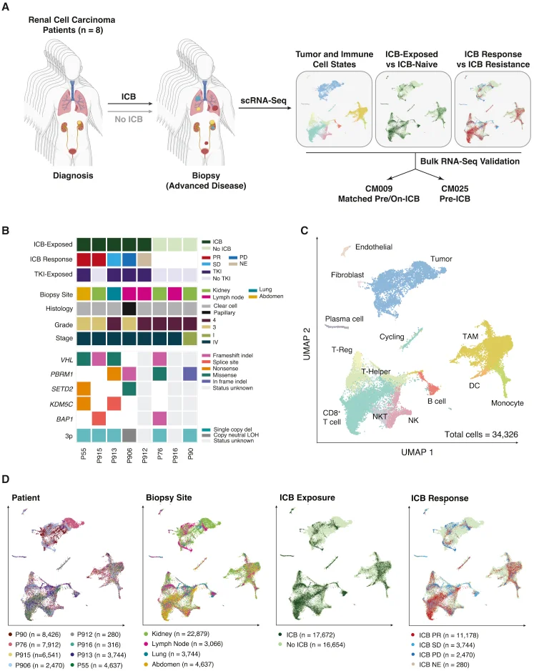
Characterizing the tumor microenvironment of advanced RCC during therapy (A) Study overview. (B) Summary of treatment histories at time of biopsy, clinicopathological features, and genomic features across profiled RCC lesions. ICB Response: PR, partial response; SD, stable disease; PD, progressive disease; NE, not evaluable. For some samples without successful whole-exome sequencing, genomic characterization is incomplete or missing. (C) Uniform manifold approximation and projection (UMAP) of malignant and non-malignant cells captured across all lesions, colored by broad cell type. Granular cell types and states were discerned through iterative reprojection and unsupervised clustering of lymphoid, myeloid, and tumor compartments, and merged into broader cell-type categories for this visualization. DC, dendritic cell; NK, natural killer cell; NKT, natural killer T cell; TAM, tumor-associated macrophage; T-Reg, regulatory T cell. (D) UMAP of malignant and non-malignant cells captured across all lesions, colored by patient, biopsy site, ICB treatment history, and ICB response. See also Figure S1 , Table S1 .

Figure 1 from Kevin Bi et al., Cancer Cell (2021). Licensed CC BY-NC-ND. Source: 10.1016/j.ccell.2021.02.015.

Cancer Cell (2021) · 542 citations

Read the original → https://doi.org/10.1016/j.ccell.2021.02.015


Microenvironment drives cell state, plasticity, and drug response in pancreatic cancer

This study profiled pancreatic cancer tumors and matching lab-grown organoids at single-cell resolution, showing that the surrounding tissue environment strongly shapes cancer cell behavior and drug response. It also finds that lab models can distort cancer cell states, and that restoring certain signals helps preserve their original diversity.
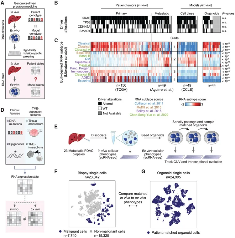
Assessing transcriptional states in patient tumors and cancer models (A) Precision medicine pipelines assess model fidelity for genetics but typically do not evaluate RNA states. (B) Alterations in PDAC driver genes across primary resections (TCGA), metastatic biopsies (Panc-Seq), and organoid and cell line (CCLE) models. Grey indicates where genomic data were not available. P -values by Fisher’s exact test. (C) Comparison of PDAC expression signatures from bulk RNA-sequencing in primary and metastatic tumors, cell lines, and organoid models in (B). Rows are clustered, columns are sorted by average basal-classical score difference. P -values indicate differences between patient tumors, cell lines, and organoids by ANOVA. (D) Schematic of contributors to RNA state that may lead to differences between in vivo and ex vivo expression patterns. (E) Metastatic patient samples were collected via core needle biopsies and dissociated. Biopsy cells were allocated for scRNA-seq, and patient-matched organoids were developed with downstream serial scRNA-seq sampling. (F and G) t -distributed stochastic neighbor embedding ( t -SNE) for biopsy (F) and matched patient-derived organoid cells (G). See also Figure S1 ; Tables S1 and S2 .

Figure 1 from Srivatsan Raghavan et al., Cell (2021). Licensed CC BY-NC-ND. Source: 10.1016/j.cell.2021.11.017.

Cell (2021) · 493 citations

Read the original → https://doi.org/10.1016/j.cell.2021.11.017


SSMGCN: Multi-View Graph Clustering with Shared-Specific Information Modelling for Spatially Resolved Transcriptomics.

A new method called SSMGCN improves the identification of spatial regions in tissue samples by combining two types of biological graphs and separating shared from unique information. The goal is to make spatial transcriptomics analyses less sensitive to the choice of similarity metric, which has been a pain point in complex tissues.

Conceptual illustration for: SSMGCN: Multi-View Graph Clustering with Shared-Specific Information Modelling for Spatially Resolved Transcriptomics.

IEEE transactions on computational biology and bioinformatics (2026)

Read the original → https://doi.org/10.1109/tcbbio.2026.3733661


Ten quick tips for spatial transcriptomics analysis.

This practical guide walks researchers through ten key decisions for analyzing spatial transcriptomics data, from choosing the right experimental platform to interpreting results. It's aimed at newcomers trying to get a handle on a fast-growing field with many tools and data types.
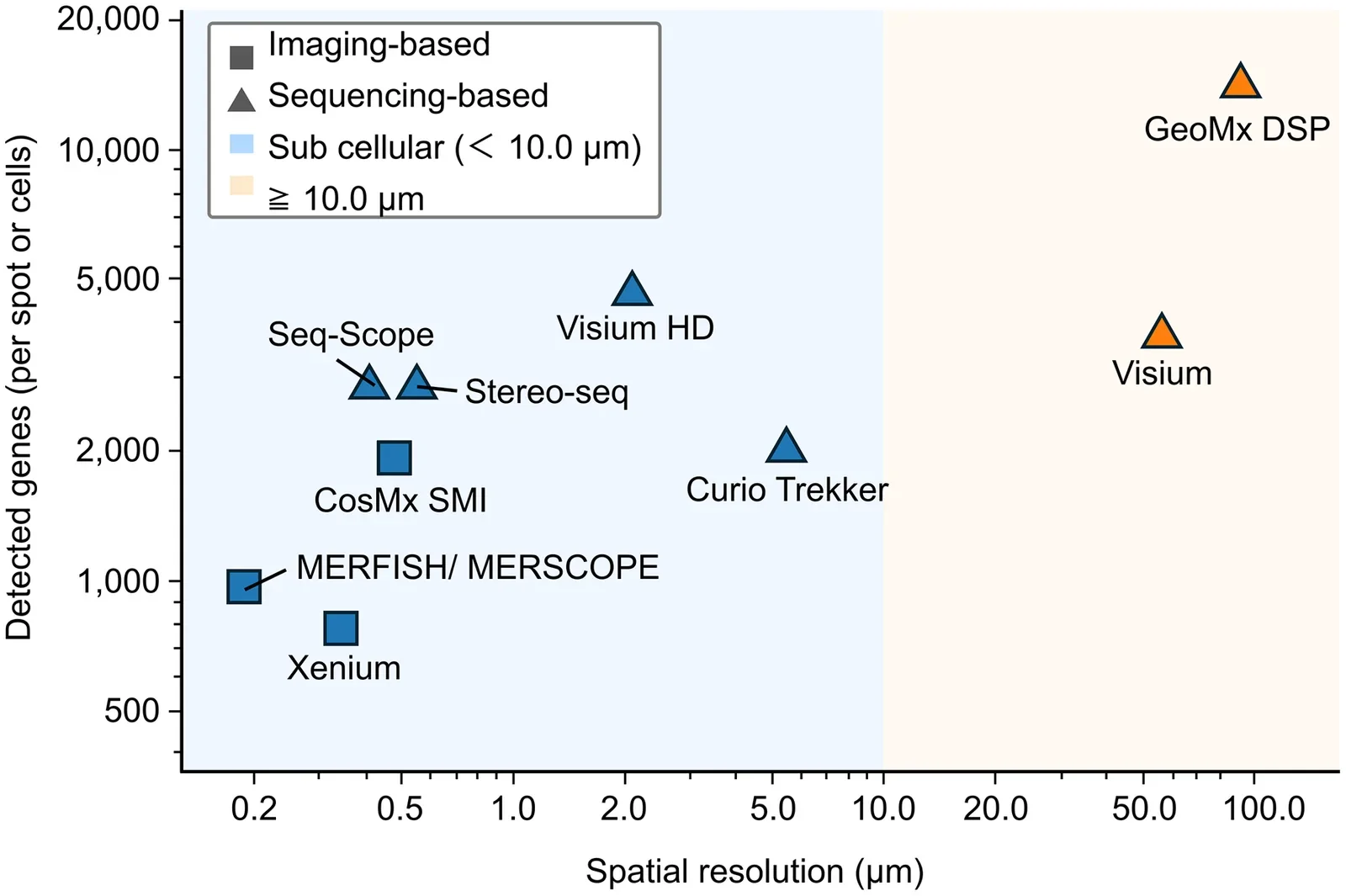
Spatial transcriptomics platforms compared by spatial resolution and transcriptome coverage. Imaging-based platforms and sequencing-based platforms are plotted by spatial resolution (x-axis, µm) versus the number of genes detected per spot or cell (y-axis). The same two-family classification is used in Table 1 . Representative imaging-based methods include smFISH, seqFISH, MERFISH/MERSCOPE, CosMx SMI, and Xenium; representative sequencing-based methods include Visium, Visium HD, Slide-seq, Stereo-seq, Seq-Scope, Curio Trekker, and GeoMx DSP. Shading distinguishes subcellular resolution (<10 µm) from resolution ≥10 µm.

Fig 1 from Kurogi N et al., PLoS computational biology (2026). Licensed CC BY. Source: 10.1371/journal.pcbi.1014757.

PLoS computational biology (2026)

Read the original → https://doi.org/10.1371/journal.pcbi.1014757


Quick links

Paper Venue / Year Link
CpG hypermethylation and WNT/AP-1 cooperativity define the epigenetic landscape and a clinical subgroup of high-risk pediatric adrenocortical carcinoma. Nature communications (2026) Read →
A microprotein atlas of the human frontal cortex in Alzheimer's disease. Nature aging (2026) Read →
Tumor and immune reprogramming during immunotherapy in advanced renal cell carcinoma Cancer Cell (2021) Read →
Microenvironment drives cell state, plasticity, and drug response in pancreatic cancer Cell (2021) Read →
SSMGCN: Multi-View Graph Clustering with Shared-Specific Information Modelling for Spatially Resolved Transcriptomics. IEEE transactions on computational biology and bioinformatics (2026) Read →
Ten quick tips for spatial transcriptomics analysis. PLoS computational biology (2026) Read →

Single-Cell Transcriptomics scRNA-seq Genomics Cancer Oncology Tumor Spatial Transcriptomics