Learning Single-Cell Analysis with Theis Lab: Bridging the Batch Gap (Part 2)

Single-Cell Best Practices

Data Integration (Part 2)

SECTION PREVIEW

1. How does BBKNN achieve lightning-fast integration through its clever "neighbor graph modification" strategy?

2. As a classic method, how does Seurat v3 MNN correct expression matrices by identifying "anchor" cells?

3. How do you use the scib package to quantitatively score integration quality?

4. Faced with different data types and analytical goals, how do you choose the right integration method for your situation?

This section corresponds to Chapters 12.7–12.10 (Integration) of the original textbook.

In the world of single-cell RNA sequencing, batch effects are a core challenge that nearly every analyst encounters. When we want to integrate data from different experimental batches, different donors, or even different laboratories to gain a more comprehensive biological picture, effectively removing batch effects—letting the data "find common ground while preserving differences"—becomes the make-or-break step of the entire analysis. This article provides a systematic introduction to the principles, methods, and practical implementation of single-cell data integration.

See Learning Single-Cell Analysis with Theis Lab: Bridging the Batch Gap (Part 1) for the first part of this series.

Graph-Based Integration: BBKNN

BBKNN (Batch Balanced k-Nearest Neighbors) takes a distinctly different approach to integration. Rather than generating a batch-corrected low-dimensional embedding or expression matrix, it intervenes directly at the k-nearest neighbor (kNN) graph construction stage.

Core Principle

The standard kNN algorithm searches the entire dataset to find the most similar neighbors for each cell. When strong batch effects are present, this almost inevitably results in cells preferentially connecting to neighbors from their own batch. BBKNN's key innovation is to search for nearest neighbors within each batch separately, then merge these cross-batch neighbors together—forcibly creating connections between different batches.

This seemingly simple modification is remarkably effective at handling strong batch effects.

import bbknn

# Use the batch-aware HVG data
adata_bbknn = adata_hvg.copy()

# BBKNN operates on PCA-reduced space
sc.tl.pca(adata_bbknn)

# Run BBKNN integration
# Recommendation: use neighbors_within_batch=25 for >100,000 cells; use 3 otherwise
neighbors_within_batch = 3 if adata_hvg.n_obs < 100000 else 25

bbknn.bbknn(
    adata_bbknn,
    batch_key=batch_key,
    neighbors_within_batch=neighbors_within_batch
)

# Compute UMAP directly from the BBKNN-integrated neighbor graph
sc.tl.umap(adata_bbknn)
sc.pl.umap(
    adata_bbknn,
    color=[label_key, batch_key],
    wspace=0.5,
    title=["Cell Type (BBKNN integrated)", "Batch (BBKNN integrated)"]
)

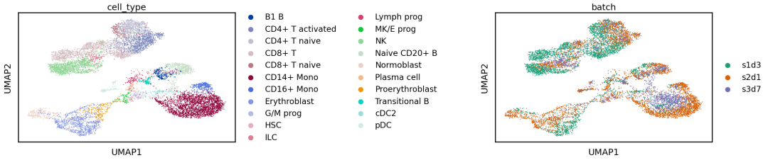BBKNN integration results

BBKNN's greatest strength is its speed—it's ideal for rapid exploration in the early stages of an analysis. Its limitation is equally clear: because it only outputs an integrated graph structure, it cannot be used for downstream analyses that require a batch-corrected expression matrix (e.g., differential expression analysis).

Linear Embedding Integration: Seurat v3 (MNN)

Seurat v3's integration strategy is built on the concepts of anchors and Mutual Nearest Neighbors (MNNs). Briefly, MNNs are pairs of cells—one from each batch—that are each other's nearest neighbors in the dimensionality-reduced space. Seurat v3 treats these MNN pairs as representing the same cell state across batches and uses them as "anchors."

The integration process involves two steps:

1. Find anchors: Identify a sufficient number of MNN pairs across batches.
2. Integrate data: Compute a correction vector from the anchors to "align" one batch onto another, ultimately outputting an integrated gene expression matrix.

Since Seurat is an R package, we need tools to pass data between Python and R.

1. Data preparation in Python

# Use HVG data
adata_seurat = adata_hvg.copy()

# Ensure batch and cell type columns are string format for R compatibility
adata_seurat.obs[batch_key] = adata_seurat.obs[batch_key].astype(str)
adata_seurat.obs[label_key] = adata_seurat.obs[label_key].astype(str)

# Remove complex objects from uns that may cause conversion failures
del adata_seurat.uns

2. Calling R via the rpy2 interface

%%R -i adata_seurat -o integrated_expr

library(Seurat)
# Convert AnnData object to a Seurat object
seurat_obj <- as.Seurat(adata_seurat, counts = "X", data = NULL)

# Split into a list by batch
batch_list <- SplitObject(seurat_obj, split.by = batch_key)

# Find integration anchors
anchors <- FindIntegrationAnchors(
    object.list = batch_list,
    anchor.features = rownames(batch_list[[1]])  # Use all HVGs as features
)

# Integrate data using anchors
integrated <- IntegrateData(anchorset = anchors)

# Extract the corrected expression matrix
integrated_expr <- GetAssayData(integrated, assay = "integrated", slot = "data")

# Transpose to conform to AnnData format (cells × genes)
integrated_expr <- t(integrated_expr)

3. Back in Python: store results and visualize

# Store the corrected matrix returned from R in the AnnData object
adata_seurat.obsm["X_seurat"] = integrated_expr.copy()

# Recompute PCA and UMAP
sc.pp.neighbors(adata_seurat, use_rep="X_seurat")
sc.tl.umap(adata_seurat)
sc.pl.umap(
    adata_seurat,
    color=[label_key, batch_key],
    wspace=0.5,
    title=["Cell Type (Seurat integrated)", "Batch (Seurat integrated)"]
)

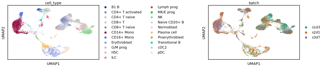Seurat MNN integration results

Seurat v3's strength lies in producing a corrected, interpretable gene expression matrix—critical for downstream tasks like differential expression analysis. It is very reliable for handling straightforward batch effects.

Quantitative Evaluation of Integration Quality

Judging integration quality from UMAP plots alone is far from sufficient, as visual inspection can be misleading. A truly good integration should simultaneously achieve two goals:

1. Batch correction: Mix cells from different batches as thoroughly as possible, eliminating technical differences.
2. Biological structure preservation: Maintain cell type distinctions without destroying true biological heterogeneity.

We need quantitative metrics to measure both dimensions. The scib (single-cell integration benchmarking) package provides a standardized evaluation framework for exactly this purpose.

Running a quick evaluation with scib

import scib

# Compute a battery of evaluation metrics for each integration method
# Note: we pass both the original data (adata) and the integrated data for comparison

# Unintegrated data as baseline
metrics_hvg = scib.metrics.metrics_fast(
    adata, adata_hvg, batch_key, label_key, embed="X_pca"
)
# scVI
metrics_scvi = scib.metrics.metrics_fast(
    adata, adata_scvi, batch_key, label_key, embed="X_scVI"
)
# scANVI
metrics_scanvi = scib.metrics.metrics_fast(
    adata, adata_scanvi, batch_key, label_key, embed="X_scANVI"
)
# BBKNN (evaluated in PCA space)
metrics_bbknn = scib.metrics.metrics_fast(
    adata, adata_bbknn, batch_key, label_key, embed='X_pca', type_='graph'
)
# Seurat
metrics_seurat = scib.metrics.metrics_fast(
    adata, adata_seurat, batch_key, label_key, embed="X_seurat"
)

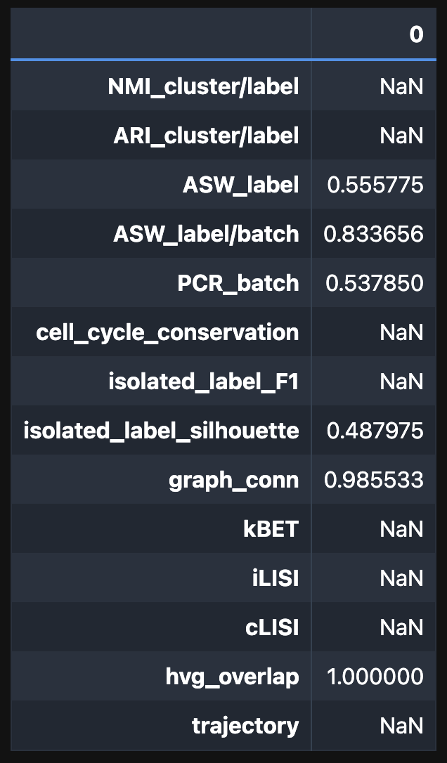Results for a single method

Aggregating and visualizing all evaluation results

import pandas as pd

# Combine all results into a single DataFrame
metrics = pd.concat(
    [metrics_scvi, metrics_scanvi, metrics_bbknn,
     metrics_seurat, metrics_hvg],
    axis="columns"
)
metrics.columns = ["scVI", "scANVI", "BBKNN", "Seurat", "Unintegrated"]

# Select a few key metrics for visualization
metrics_plot = metrics.loc[
    ["ASW_label", "NMI", "PCR_batch", "graph_conn", "kBET"], :
].T

# Scale metrics to [0, 1] for easy comparison and composite scoring
metrics_scaled = (metrics_plot - metrics_plot.min()) / (metrics_plot.max() - metrics_plot.min())

# Compute composite scores (weights can be adjusted based on your priorities)
# Biological conservation metrics (60% weight)
bio_metrics = ["ASW_label", "NMI"]
# Batch correction metrics (40% weight)
batch_metrics = ["PCR_batch", "graph_conn", "kBET"]

metrics_scaled["Bio conservation"] = metrics_scaled[bio_metrics].mean(axis=1)
metrics_scaled["Batch correction"] = metrics_scaled[batch_metrics].mean(axis=1)

# Final composite score
metrics_scaled["Overall score"] = 0.6 * metrics_scaled["Bio conservation"] + 0.4 * metrics_scaled["Batch correction"]

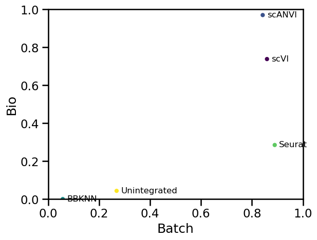
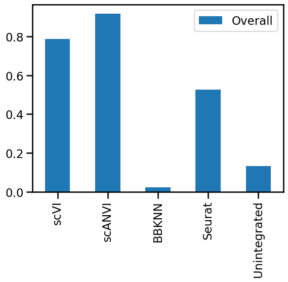
# Plot a bar chart comparing overall scores
metrics_scaled.sort_values("Overall score", ascending=False).plot.bar(
    y="Overall score", legend=None
)

★

Editor's note: The weight allocation in the scib evaluation framework (e.g., 60% biological conservation vs. 40% batch correction) is an empirical choice. Feel free to adjust it based on your project's core goals. If you're primarily building a seamless cell atlas, you might give more weight to "batch correction." Conversely, if your goal is to identify novel, rare cell subpopulations, "biological conservation" should carry more weight.

Interpreting the key metrics (higher is better, except for kBET):

• Biological conservation:
  • NMI (Normalized Mutual Information): Compares cell type clustering before and after integration; measures how well cell type labels are preserved.
  • ASW_label (Average Silhouette Width by label): Measures whether cells of the same type cluster tightly together.
• Batch correction:
  • PCR_batch (Principal Component Regression by batch): Measures what fraction of variance in the integrated principal components can still be explained by batch. A higher score means batch explains less variance—i.e., better correction.
  • graph_conn (Graph connectivity): Measures whether cells of the same type from different batches are connected in the integrated graph.
  • kBET (lower is better): Measures the degree of batch mixing in local neighborhoods.

Based on the results, scANVI and scVI achieved the highest composite scores on this benchmark, demonstrating strong balance between batch correction and biological preservation.

Definitive Recommendations for Method Selection

No single integration method is universally optimal. The right choice depends on your dataset size, complexity, and analytical goals.

Scenario / Need	Recommended Method	Notes
Large datasets (>100k cells)	scVI / scANVI	Excellent scalability; handles massive datasets efficiently
Simple batch correction (same technology platform, different batches)	Harmony, Seurat v3	Fast, reliable, easy to use
Complex integration (cross-technology, cross-species)	scVI / scANVI, Scanorama	Can handle nonlinear, complex batch effects
Need a corrected expression matrix	Seurat v3, scVI (reconstructable)	Essential for downstream analyses like differential expression
Rapid exploratory analysis	BBKNN	Fastest method; great for an initial look at integration potential

Practical tips from experience:

1. Look before you leap: Before integrating, always assess the strength of batch effects in your raw data using PCA or UMAP. Mild effects may not require correction at all.
2. Compare multiple methods: For important projects, try 2–3 different types of integration methods and use scib for quantitative comparison.
3. Parameters are not set in stone: All methods have tunable parameters. Defaults are a good starting point, but fine-tuning for your specific data can yield better results.
4. Come back to the biology: After integration, always check that the expression patterns of known cell type marker genes look correct. Verify that integration hasn't introduced or eliminated critical biological signals.

Key Takeaways

• Batch effects are ubiquitous, but before integrating, you must think clearly about which variation is technical noise to remove and which is biological signal to preserve.
• Methods have different strengths:
  • Deep learning (scVI/scANVI): The go-to for complex, large-scale datasets.
  • Linear embedding (Seurat/Harmony): Reliable workhorses for simpler tasks.
  • Graph-based (BBKNN): The speed champion for exploratory analysis.
• Quantitative evaluation is the gold standard: Never trust your eyes (UMAP) alone. Use tools like scib to evaluate both "batch correction" and "biological conservation" rigorously.
• There is no one-size-fits-all solution: The best method is always the one that best fits your data characteristics, analytical goals, and computational resources.

Closing Thoughts

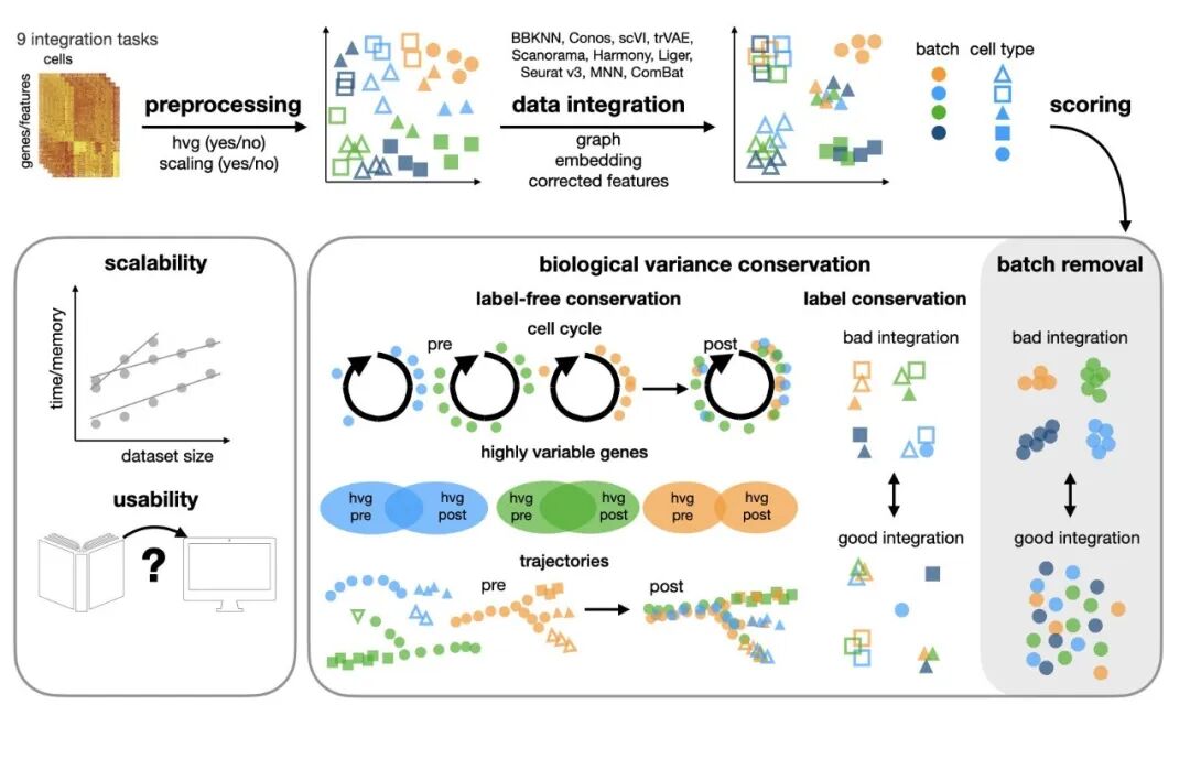
scib is a Python package developed by the Theis Lab for evaluating integration performance. It encompasses many commonly used criteria, including graph connectivity and label consistency. One particularly clever feature is that you can customize the weighting between batch effect removal and the biological diversity inherent to your samples—allowing for a more nuanced balance. Interested readers can find more details on GitHub (theislab/scib) and in the paper Benchmarking atlas-level data integration in single-cell genomics.

Source: scib GitHub repository

What's your take on batch correction? Which tools work best, and which ones tend to overfit? Share your experiences in the comments!

The Bioinfo Study Room discussion group welcomes all bioinformatics enthusiasts:

---

Originally posted on WeChat Official Account: bioinfo_studyroom